Feature Engineering and Polynomial Regression
- 1. 多项式特征
- 2. 选择特征
- 3. 缩放特征
- 4. 复杂函数
- 附录
首先,导入所需的库:
import numpy as np
import matplotlib.pyplot as plt
from lab_utils_multi import zscore_normalize_features, run_gradient_descent_feng
np.set_printoptions(precision=2)  # reduced display precision on numpy arrays
线性回归模型表示为:
f w , b = w 0 x 0 + w 1 x 1 + . . . + w n − 1 x n − 1 + b (1) f_{\mathbf{w},b} = w_0x_0 + w_1x_1+ ... + w_{n-1}x_{n-1} + b \tag{1} fw,b=w0x0+w1x1+...+wn−1xn−1+b(1)
思考一下,如果特征是非线性的或者是特征的结合,线性模型不能拟合,那该怎么办?
1. 多项式特征
尝试使用目前已知的知识来拟合非线性曲线。我们将从一个简单的二次方程开始: y = 1 + x 2 y = 1+x^2 y=1+x2
# create target data
x = np.arange(0, 20, 1)
y = 1 + x**2
X = x.reshape(-1, 1)model_w,model_b = run_gradient_descent_feng(X,y,iterations=1000, alpha = 1e-2)plt.scatter(x, y, marker='x', c='r', label="Actual Value"); plt.title("no feature engineering")
plt.plot(x,X@model_w + model_b, label="Predicted Value");  plt.xlabel("X"); plt.ylabel("y"); plt.legend(); plt.show()
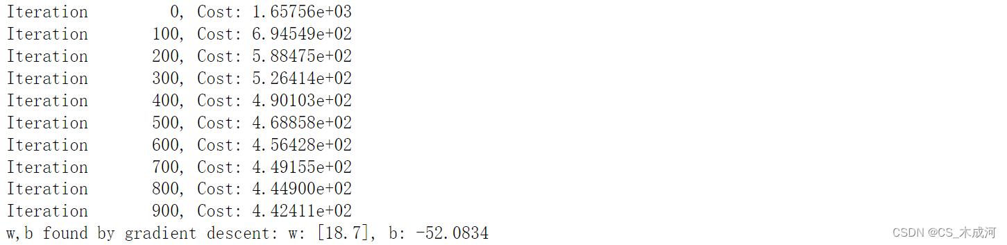
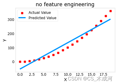
正如所期待的那样,线性方程明显不合适。如果将X 换成 X**2会如何?
# create target data
x = np.arange(0, 20, 1)
y = 1 + x**2# Engineer features
X = x**2      #<-- added engineered feature
X = X.reshape(-1, 1)  #X should be a 2-D Matrix
model_w,model_b = run_gradient_descent_feng(X, y, iterations=10000, alpha = 1e-5)plt.scatter(x, y, marker='x', c='r', label="Actual Value"); plt.title("Added x**2 feature")
plt.plot(x, np.dot(X,model_w) + model_b, label="Predicted Value"); plt.xlabel("x"); plt.ylabel("y"); plt.legend(); plt.show()
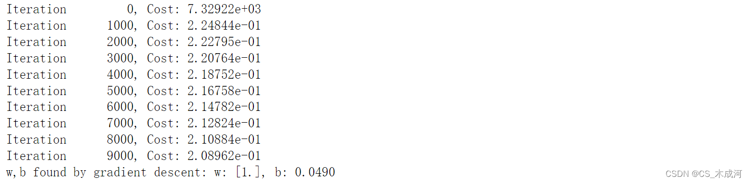
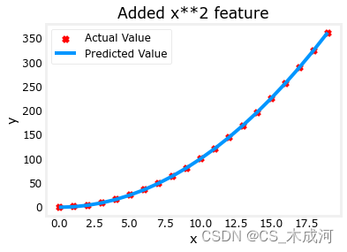
梯度下降将 w , b \mathbf{w},b w,b的初始值修改为 (1.0,0.049) ,即模型方程 y = 1 ∗ x 0 2 + 0.049 y=1*x_0^2+0.049 y=1∗x02+0.049, 这非常接近目标方程 y = 1 ∗ x 0 2 + 1 y=1*x_0^2+1 y=1∗x02+1.
2. 选择特征
从上面可以知道, x 2 x^2 x2是需要的。接下来我们尝试: y = w 0 x 0 + w 1 x 1 2 + w 2 x 2 3 + b y=w_0x_0 + w_1x_1^2 + w_2x_2^3+b y=w0x0+w1x12+w2x23+b
# create target data
x = np.arange(0, 20, 1)
y = x**2# engineer features .
X = np.c_[x, x**2, x**3]   #<-- added engineered feature
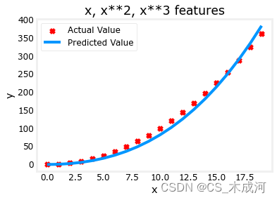
model_w,model_b = run_gradient_descent_feng(X, y, iterations=10000, alpha=1e-7)plt.scatter(x, y, marker='x', c='r', label="Actual Value"); plt.title("x, x**2, x**3 features")
plt.plot(x, X@model_w + model_b, label="Predicted Value"); plt.xlabel("x"); plt.ylabel("y"); plt.legend(); plt.show()
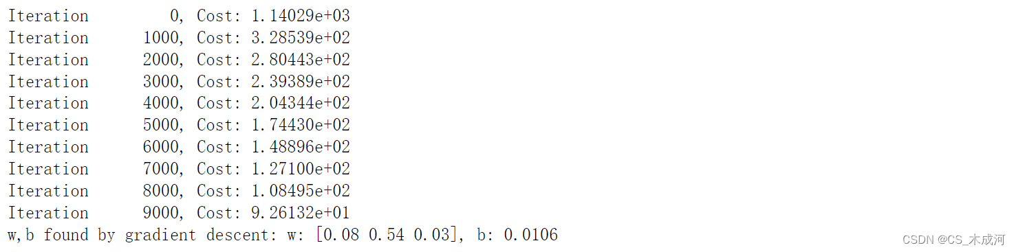
w \mathbf{w} w的值为 [0.08 0.54 0.03] , b 为 0.0106。训练后的模型为:
0.08 x + 0.54 x 2 + 0.03 x 3 + 0.0106 0.08x + 0.54x^2 + 0.03x^3 + 0.0106 0.08x+0.54x2+0.03x3+0.0106
梯度下降通过相对于其他项增加 w 1 w_1 w1项,强调了最适合 x 2 x^2 x2的数据。如果运行很长时间,它将继续减少其他项的影响。梯度下降通过强调其相关参数来为我们选择“正确”的特征。
- 一般来讲,特征被重新缩放,因此它们可以相互比较
- 权重值越小意味着不太重要的特征,在极端情况下,当权重变为零或非常接近零时,相关特征在将模型拟合到数据中是有用的。
- 如上所述,拟合后,与 x 2 x^2 x2功能相关的权重远大于 x x x或 x 3 x^3 x3的权重,因为它在拟合数据时最有用。
多项式特征是根据它们与目标数据的匹配程度来选择的。一旦我们创建了新特征,我们仍然使用线性回归。最好的特征将相对于目标呈线性关系。下面通过一个例子来理解这一点。
# create target data
x = np.arange(0, 20, 1)
y = x**2# engineer features .
X = np.c_[x, x**2, x**3]   #<-- added engineered feature
X_features = ['x','x^2','x^3']
fig,ax=plt.subplots(1, 3, figsize=(12, 3), sharey=True)
for i in range(len(ax)):ax[i].scatter(X[:,i],y)ax[i].set_xlabel(X_features[i])
ax[0].set_ylabel("y")
plt.show()
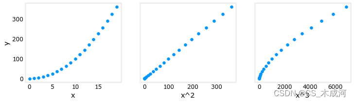
很明显, x 2 x^2 x2特征映射到目标值 y y y是线性的。线性回归可以使用该特征轻松生成模型。
3. 缩放特征
如果数据集具有显着不同尺度的特征,则应该应用特征缩放来加速梯度下降。在上面的例子中,有 x x x, x 2 x^2 x2 和 x 3 x^3 x3,这自然会有非常不同的规模。接下来将 Z-score 归一化应用到示例中。
# create target data
x = np.arange(0,20,1)
X = np.c_[x, x**2, x**3]
print(f"Peak to Peak range by column in Raw        X:{np.ptp(X,axis=0)}")# add mean_normalization
X = zscore_normalize_features(X)
print(f"Peak to Peak range by column in Normalized X:{np.ptp(X,axis=0)}")

使用更大的alpha值运行:
x = np.arange(0,20,1)
y = x**2X = np.c_[x, x**2, x**3]
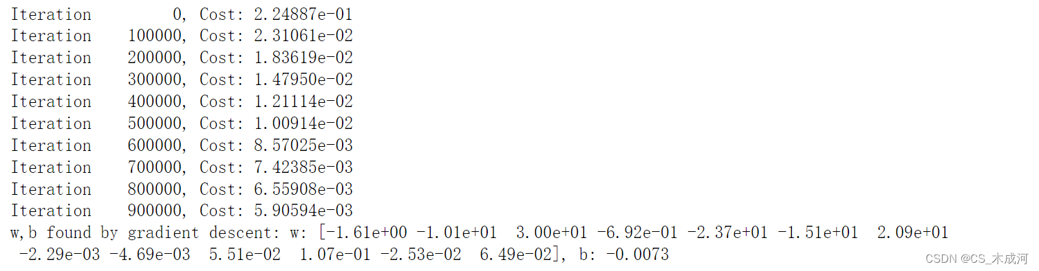
X = zscore_normalize_features(X) model_w, model_b = run_gradient_descent_feng(X, y, iterations=100000, alpha=1e-1)plt.scatter(x, y, marker='x', c='r', label="Actual Value"); plt.title("Normalized x x**2, x**3 feature")
plt.plot(x,X@model_w + model_b, label="Predicted Value"); plt.xlabel("x"); plt.ylabel("y"); plt.legend(); plt.show()
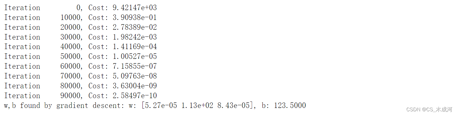
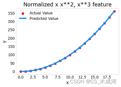
特征缩放使得收敛速度更快。梯度下降过程中, x 2 x^2 x2 是最受强调的, x 3 x^3 x3项几乎被消除。
4. 复杂函数
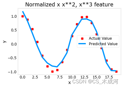
通过特征工程,甚至可以对相当复杂的函数进行建模:
x = np.arange(0,20,1)
y = np.cos(x/2)X = np.c_[x, x**2, x**3,x**4, x**5, x**6, x**7, x**8, x**9, x**10, x**11, x**12, x**13]
X = zscore_normalize_features(X) model_w,model_b = run_gradient_descent_feng(X, y, iterations=1000000, alpha = 1e-1)plt.scatter(x, y, marker='x', c='r', label="Actual Value"); plt.title("Normalized x x**2, x**3 feature")
plt.plot(x,X@model_w + model_b, label="Predicted Value"); plt.xlabel("x"); plt.ylabel("y"); plt.legend(); plt.show()
附录
lab_utils_multi.py源码:
import numpy as np
import copy
import math
from scipy.stats import norm
import matplotlib.pyplot as plt
from mpl_toolkits.mplot3d import axes3d
from matplotlib.ticker import MaxNLocator
dlblue = '#0096ff'; dlorange = '#FF9300'; dldarkred='#C00000'; dlmagenta='#FF40FF'; dlpurple='#7030A0';
plt.style.use('./deeplearning.mplstyle')def load_data_multi():data = np.loadtxt("data/ex1data2.txt", delimiter=',')X = data[:,:2]y = data[:,2]return X, y##########################################################
# Plotting Routines
##########################################################def plt_house_x(X, y,f_wb=None, ax=None):''' plot house with aXis '''if not ax:fig, ax = plt.subplots(1,1)ax.scatter(X, y, marker='x', c='r', label="Actual Value")ax.set_title("Housing Prices")ax.set_ylabel('Price (in 1000s of dollars)')ax.set_xlabel(f'Size (1000 sqft)')if f_wb is not None:ax.plot(X, f_wb,  c=dlblue, label="Our Prediction")ax.legend()def mk_cost_lines(x,y,w,b, ax):''' makes vertical cost lines'''cstr = "cost = (1/2m)*1000*("ctot = 0label = 'cost for point'for p in zip(x,y):f_wb_p = w*p[0]+bc_p = ((f_wb_p - p[1])**2)/2c_p_txt = c_p/1000ax.vlines(p[0], p[1],f_wb_p, lw=3, color=dlpurple, ls='dotted', label=label)label='' #just onecxy = [p[0], p[1] + (f_wb_p-p[1])/2]ax.annotate(f'{c_p_txt:0.0f}', xy=cxy, xycoords='data',color=dlpurple, xytext=(5, 0), textcoords='offset points')cstr += f"{c_p_txt:0.0f} +"ctot += c_pctot = ctot/(len(x))cstr = cstr[:-1] + f") = {ctot:0.0f}"ax.text(0.15,0.02,cstr, transform=ax.transAxes, color=dlpurple)def inbounds(a,b,xlim,ylim):xlow,xhigh = xlimylow,yhigh = ylimax, ay = abx, by = bif (ax > xlow and ax < xhigh) and (bx > xlow and bx < xhigh) \and (ay > ylow and ay < yhigh) and (by > ylow and by < yhigh):return(True)else:return(False)from mpl_toolkits.mplot3d import axes3d
def plt_contour_wgrad(x, y, hist, ax, w_range=[-100, 500, 5], b_range=[-500, 500, 5], contours = [0.1,50,1000,5000,10000,25000,50000], resolution=5, w_final=200, b_final=100,step=10 ):b0,w0 = np.meshgrid(np.arange(*b_range),np.arange(*w_range))z=np.zeros_like(b0)n,_ = w0.shapefor i in range(w0.shape[0]):for j in range(w0.shape[1]):z[i][j] = compute_cost(x, y, w0[i][j], b0[i][j] )CS = ax.contour(w0, b0, z, contours, linewidths=2,colors=[dlblue, dlorange, dldarkred, dlmagenta, dlpurple]) ax.clabel(CS, inline=1, fmt='%1.0f', fontsize=10)ax.set_xlabel("w");  ax.set_ylabel("b")ax.set_title('Contour plot of cost J(w,b), vs b,w with path of gradient descent')w = w_final; b=b_finalax.hlines(b, ax.get_xlim()[0],w, lw=2, color=dlpurple, ls='dotted')ax.vlines(w, ax.get_ylim()[0],b, lw=2, color=dlpurple, ls='dotted')base = hist[0]for point in hist[0::step]:edist = np.sqrt((base[0] - point[0])**2 + (base[1] - point[1])**2)if(edist > resolution or point==hist[-1]):if inbounds(point,base, ax.get_xlim(),ax.get_ylim()):plt.annotate('', xy=point, xytext=base,xycoords='data',arrowprops={'arrowstyle': '->', 'color': 'r', 'lw': 3},va='center', ha='center')base=pointreturn# plots p1 vs p2. Prange is an array of entries [min, max, steps]. In feature scaling lab.
def plt_contour_multi(x, y, w, b, ax, prange, p1, p2, title="", xlabel="", ylabel=""): contours = [1e2, 2e2,3e2,4e2, 5e2, 6e2, 7e2,8e2,1e3, 1.25e3,1.5e3, 1e4, 1e5, 1e6, 1e7]px,py = np.meshgrid(np.linspace(*(prange[p1])),np.linspace(*(prange[p2])))z=np.zeros_like(px)n,_ = px.shapefor i in range(px.shape[0]):for j in range(px.shape[1]):w_ij = wb_ij = bif p1 <= 3: w_ij[p1] = px[i,j]if p1 == 4: b_ij = px[i,j]if p2 <= 3: w_ij[p2] = py[i,j]if p2 == 4: b_ij = py[i,j]z[i][j] = compute_cost(x, y, w_ij, b_ij )CS = ax.contour(px, py, z, contours, linewidths=2,colors=[dlblue, dlorange, dldarkred, dlmagenta, dlpurple]) ax.clabel(CS, inline=1, fmt='%1.2e', fontsize=10)ax.set_xlabel(xlabel);  ax.set_ylabel(ylabel)ax.set_title(title, fontsize=14)def plt_equal_scale(X_train, X_norm, y_train):fig,ax = plt.subplots(1,2,figsize=(12,5))prange = [[ 0.238-0.045, 0.238+0.045,  50],[-25.77326319-0.045, -25.77326319+0.045, 50],[-50000, 0,      50],[-1500,  0,      50],[0, 200000, 50]]w_best = np.array([0.23844318, -25.77326319, -58.11084634,  -1.57727192])b_best = 235plt_contour_multi(X_train, y_train, w_best, b_best, ax[0], prange, 0, 1, title='Unnormalized, J(w,b), vs w[0],w[1]',xlabel= "w[0] (size(sqft))", ylabel="w[1] (# bedrooms)")#w_best = np.array([111.1972, -16.75480051, -28.51530411, -37.17305735])b_best = 376.949151515151prange = [[ 111-50, 111+50,   75],[-16.75-50,-16.75+50, 75],[-28.5-8, -28.5+8,  50],[-37.1-16,-37.1+16, 50],[376-150, 376+150, 50]]plt_contour_multi(X_norm, y_train, w_best, b_best, ax[1], prange, 0, 1, title='Normalized, J(w,b), vs w[0],w[1]',xlabel= "w[0] (normalized size(sqft))", ylabel="w[1] (normalized # bedrooms)")fig.suptitle("Cost contour with equal scale", fontsize=18)#plt.tight_layout(rect=(0,0,1.05,1.05))fig.tight_layout(rect=(0,0,1,0.95))plt.show()def plt_divergence(p_hist, J_hist, x_train,y_train):x=np.zeros(len(p_hist))y=np.zeros(len(p_hist))v=np.zeros(len(p_hist))for i in range(len(p_hist)):x[i] = p_hist[i][0]y[i] = p_hist[i][1]v[i] = J_hist[i]fig = plt.figure(figsize=(12,5))plt.subplots_adjust( wspace=0 )gs = fig.add_gridspec(1, 5)fig.suptitle(f"Cost escalates when learning rate is too large")#===============#  First subplot#===============ax = fig.add_subplot(gs[:2], )# Print w vs cost to see minimumfix_b = 100w_array = np.arange(-70000, 70000, 1000)cost = np.zeros_like(w_array)for i in range(len(w_array)):tmp_w = w_array[i]cost[i] = compute_cost(x_train, y_train, tmp_w, fix_b)ax.plot(w_array, cost)ax.plot(x,v, c=dlmagenta)ax.set_title("Cost vs w, b set to 100")ax.set_ylabel('Cost')ax.set_xlabel('w')ax.xaxis.set_major_locator(MaxNLocator(2)) #===============# Second Subplot#===============tmp_b,tmp_w = np.meshgrid(np.arange(-35000, 35000, 500),np.arange(-70000, 70000, 500))z=np.zeros_like(tmp_b)for i in range(tmp_w.shape[0]):for j in range(tmp_w.shape[1]):z[i][j] = compute_cost(x_train, y_train, tmp_w[i][j], tmp_b[i][j] )ax = fig.add_subplot(gs[2:], projection='3d')ax.plot_surface(tmp_w, tmp_b, z,  alpha=0.3, color=dlblue)ax.xaxis.set_major_locator(MaxNLocator(2)) ax.yaxis.set_major_locator(MaxNLocator(2)) ax.set_xlabel('w', fontsize=16)ax.set_ylabel('b', fontsize=16)ax.set_zlabel('\ncost', fontsize=16)plt.title('Cost vs (b, w)')# Customize the view angle ax.view_init(elev=20., azim=-65)ax.plot(x, y, v,c=dlmagenta)return# draw derivative line
# y = m*(x - x1) + y1
def add_line(dj_dx, x1, y1, d, ax):x = np.linspace(x1-d, x1+d,50)y = dj_dx*(x - x1) + y1ax.scatter(x1, y1, color=dlblue, s=50)ax.plot(x, y, '--', c=dldarkred,zorder=10, linewidth = 1)xoff = 30 if x1 == 200 else 10ax.annotate(r"$\frac{\partial J}{\partial w}$ =%d" % dj_dx, fontsize=14,xy=(x1, y1), xycoords='data',xytext=(xoff, 10), textcoords='offset points',arrowprops=dict(arrowstyle="->"),horizontalalignment='left', verticalalignment='top')def plt_gradients(x_train,y_train, f_compute_cost, f_compute_gradient):#===============#  First subplot#===============fig,ax = plt.subplots(1,2,figsize=(12,4))# Print w vs cost to see minimumfix_b = 100w_array = np.linspace(-100, 500, 50)w_array = np.linspace(0, 400, 50)cost = np.zeros_like(w_array)for i in range(len(w_array)):tmp_w = w_array[i]cost[i] = f_compute_cost(x_train, y_train, tmp_w, fix_b)ax[0].plot(w_array, cost,linewidth=1)ax[0].set_title("Cost vs w, with gradient; b set to 100")ax[0].set_ylabel('Cost')ax[0].set_xlabel('w')# plot lines for fixed b=100for tmp_w in [100,200,300]:fix_b = 100dj_dw,dj_db = f_compute_gradient(x_train, y_train, tmp_w, fix_b )j = f_compute_cost(x_train, y_train, tmp_w, fix_b)add_line(dj_dw, tmp_w, j, 30, ax[0])#===============# Second Subplot#===============tmp_b,tmp_w = np.meshgrid(np.linspace(-200, 200, 10), np.linspace(-100, 600, 10))U = np.zeros_like(tmp_w)V = np.zeros_like(tmp_b)for i in range(tmp_w.shape[0]):for j in range(tmp_w.shape[1]):U[i][j], V[i][j] = f_compute_gradient(x_train, y_train, tmp_w[i][j], tmp_b[i][j] )X = tmp_wY = tmp_bn=-2color_array = np.sqrt(((V-n)/2)**2 + ((U-n)/2)**2)ax[1].set_title('Gradient shown in quiver plot')Q = ax[1].quiver(X, Y, U, V, color_array, units='width', )qk = ax[1].quiverkey(Q, 0.9, 0.9, 2, r'$2 \frac{m}{s}$', labelpos='E',coordinates='figure')ax[1].set_xlabel("w"); ax[1].set_ylabel("b")def norm_plot(ax, data):scale = (np.max(data) - np.min(data))*0.2x = np.linspace(np.min(data)-scale,np.max(data)+scale,50)_,bins, _ = ax.hist(data, x, color="xkcd:azure")#ax.set_ylabel("Count")mu = np.mean(data); std = np.std(data); dist = norm.pdf(bins, loc=mu, scale = std)axr = ax.twinx()axr.plot(bins,dist, color = "orangered", lw=2)axr.set_ylim(bottom=0)axr.axis('off')def plot_cost_i_w(X,y,hist):ws = np.array([ p[0] for p in hist["params"]])rng = max(abs(ws[:,0].min()),abs(ws[:,0].max()))wr = np.linspace(-rng+0.27,rng+0.27,20)cst = [compute_cost(X,y,np.array([wr[i],-32, -67, -1.46]), 221) for i in range(len(wr))]fig,ax = plt.subplots(1,2,figsize=(12,3))ax[0].plot(hist["iter"], (hist["cost"]));  ax[0].set_title("Cost vs Iteration")ax[0].set_xlabel("iteration"); ax[0].set_ylabel("Cost")ax[1].plot(wr, cst); ax[1].set_title("Cost vs w[0]")ax[1].set_xlabel("w[0]"); ax[1].set_ylabel("Cost")ax[1].plot(ws[:,0],hist["cost"])plt.show()##########################################################
# Regression Routines
##########################################################def compute_gradient_matrix(X, y, w, b): """Computes the gradient for linear regression Args:X : (array_like Shape (m,n)) variable such as house size y : (array_like Shape (m,1)) actual value w : (array_like Shape (n,1)) Values of parameters of the model      b : (scalar )                Values of parameter of the model      Returnsdj_dw: (array_like Shape (n,1)) The gradient of the cost w.r.t. the parameters w. dj_db: (scalar)                The gradient of the cost w.r.t. the parameter b. """m,n = X.shapef_wb = X @ w + b              e   = f_wb - y                dj_dw  = (1/m) * (X.T @ e)    dj_db  = (1/m) * np.sum(e)    return dj_db,dj_dw#Function to calculate the cost
def compute_cost_matrix(X, y, w, b, verbose=False):"""Computes the gradient for linear regression Args:X : (array_like Shape (m,n)) variable such as house size y : (array_like Shape (m,)) actual value w : (array_like Shape (n,)) parameters of the model b : (scalar               ) parameter of the model verbose : (Boolean) If true, print out intermediate value f_wbReturnscost: (scalar)                      """ m,n = X.shape# calculate f_wb for all examples.f_wb = X @ w + b  # calculate costtotal_cost = (1/(2*m)) * np.sum((f_wb-y)**2)if verbose: print("f_wb:")if verbose: print(f_wb)return total_cost# Loop version of multi-variable compute_cost
def compute_cost(X, y, w, b): """compute costArgs:X : (ndarray): Shape (m,n) matrix of examples with multiple featuresw : (ndarray): Shape (n)   parameters for prediction   b : (scalar):              parameter  for prediction   Returnscost: (scalar)             cost"""m = X.shape[0]cost = 0.0for i in range(m):                                f_wb_i = np.dot(X[i],w) + b       cost = cost + (f_wb_i - y[i])**2              cost = cost/(2*m)                                 return(np.squeeze(cost)) def compute_gradient(X, y, w, b): """Computes the gradient for linear regression Args:X : (ndarray Shape (m,n)) matrix of examples y : (ndarray Shape (m,))  target value of each examplew : (ndarray Shape (n,))  parameters of the model      b : (scalar)              parameter of the model      Returnsdj_dw : (ndarray Shape (n,)) The gradient of the cost w.r.t. the parameters w. dj_db : (scalar)             The gradient of the cost w.r.t. the parameter b. """m,n = X.shape           #(number of examples, number of features)dj_dw = np.zeros((n,))dj_db = 0.for i in range(m):                             err = (np.dot(X[i], w) + b) - y[i]   for j in range(n):                         dj_dw[j] = dj_dw[j] + err * X[i,j]    dj_db = dj_db + err                        dj_dw = dj_dw/m                                dj_db = dj_db/m                                return dj_db,dj_dw#This version saves more values and is more verbose than the assigment versons
def gradient_descent_houses(X, y, w_in, b_in, cost_function, gradient_function, alpha, num_iters): """Performs batch gradient descent to learn theta. Updates theta by taking num_iters gradient steps with learning rate alphaArgs:X : (array_like Shape (m,n)    matrix of examples y : (array_like Shape (m,))    target value of each examplew_in : (array_like Shape (n,)) Initial values of parameters of the modelb_in : (scalar)                Initial value of parameter of the modelcost_function: function to compute costgradient_function: function to compute the gradientalpha : (float) Learning ratenum_iters : (int) number of iterations to run gradient descentReturnsw : (array_like Shape (n,)) Updated values of parameters of the model afterrunning gradient descentb : (scalar)                Updated value of parameter of the model afterrunning gradient descent"""# number of training examplesm = len(X)# An array to store values at each iteration primarily for graphing laterhist={}hist["cost"] = []; hist["params"] = []; hist["grads"]=[]; hist["iter"]=[];w = copy.deepcopy(w_in)  #avoid modifying global w within functionb = b_insave_interval = np.ceil(num_iters/10000) # prevent resource exhaustion for long runsprint(f"Iteration Cost          w0       w1       w2       w3       b       djdw0    djdw1    djdw2    djdw3    djdb  ")print(f"---------------------|--------|--------|--------|--------|--------|--------|--------|--------|--------|--------|")for i in range(num_iters):# Calculate the gradient and update the parametersdj_db,dj_dw = gradient_function(X, y, w, b)   # Update Parameters using w, b, alpha and gradientw = w - alpha * dj_dw               b = b - alpha * dj_db               # Save cost J,w,b at each save interval for graphingif i == 0 or i % save_interval == 0:     hist["cost"].append(cost_function(X, y, w, b))hist["params"].append([w,b])hist["grads"].append([dj_dw,dj_db])hist["iter"].append(i)# Print cost every at intervals 10 times or as many iterations if < 10if i% math.ceil(num_iters/10) == 0:#print(f"Iteration {i:4d}: Cost {cost_function(X, y, w, b):8.2f}   ")cst = cost_function(X, y, w, b)print(f"{i:9d} {cst:0.5e} {w[0]: 0.1e} {w[1]: 0.1e} {w[2]: 0.1e} {w[3]: 0.1e} {b: 0.1e} {dj_dw[0]: 0.1e} {dj_dw[1]: 0.1e} {dj_dw[2]: 0.1e} {dj_dw[3]: 0.1e} {dj_db: 0.1e}")return w, b, hist #return w,b and history for graphingdef run_gradient_descent(X,y,iterations=1000, alpha = 1e-6):m,n = X.shape# initialize parametersinitial_w = np.zeros(n)initial_b = 0# run gradient descentw_out, b_out, hist_out = gradient_descent_houses(X ,y, initial_w, initial_b,compute_cost, compute_gradient_matrix, alpha, iterations)print(f"w,b found by gradient descent: w: {w_out}, b: {b_out:0.2f}")return(w_out, b_out, hist_out)# compact extaction of hist data
#x = hist["iter"]
#J  = np.array([ p    for p in hist["cost"]])
#ws = np.array([ p[0] for p in hist["params"]])
#dj_ws = np.array([ p[0] for p in hist["grads"]])#bs = np.array([ p[1] for p in hist["params"]]) def run_gradient_descent_feng(X,y,iterations=1000, alpha = 1e-6):m,n = X.shape# initialize parametersinitial_w = np.zeros(n)initial_b = 0# run gradient descentw_out, b_out, hist_out = gradient_descent(X ,y, initial_w, initial_b,compute_cost, compute_gradient_matrix, alpha, iterations)print(f"w,b found by gradient descent: w: {w_out}, b: {b_out:0.4f}")return(w_out, b_out)def gradient_descent(X, y, w_in, b_in, cost_function, gradient_function, alpha, num_iters): """Performs batch gradient descent to learn theta. Updates theta by taking num_iters gradient steps with learning rate alphaArgs:X : (array_like Shape (m,n)    matrix of examples y : (array_like Shape (m,))    target value of each examplew_in : (array_like Shape (n,)) Initial values of parameters of the modelb_in : (scalar)                Initial value of parameter of the modelcost_function: function to compute costgradient_function: function to compute the gradientalpha : (float) Learning ratenum_iters : (int) number of iterations to run gradient descentReturnsw : (array_like Shape (n,)) Updated values of parameters of the model afterrunning gradient descentb : (scalar)                Updated value of parameter of the model afterrunning gradient descent"""# number of training examplesm = len(X)# An array to store values at each iteration primarily for graphing laterhist={}hist["cost"] = []; hist["params"] = []; hist["grads"]=[]; hist["iter"]=[];w = copy.deepcopy(w_in)  #avoid modifying global w within functionb = b_insave_interval = np.ceil(num_iters/10000) # prevent resource exhaustion for long runsfor i in range(num_iters):# Calculate the gradient and update the parametersdj_db,dj_dw = gradient_function(X, y, w, b)   # Update Parameters using w, b, alpha and gradientw = w - alpha * dj_dw               b = b - alpha * dj_db               # Save cost J,w,b at each save interval for graphingif i == 0 or i % save_interval == 0:     hist["cost"].append(cost_function(X, y, w, b))hist["params"].append([w,b])hist["grads"].append([dj_dw,dj_db])hist["iter"].append(i)# Print cost every at intervals 10 times or as many iterations if < 10if i% math.ceil(num_iters/10) == 0:#print(f"Iteration {i:4d}: Cost {cost_function(X, y, w, b):8.2f}   ")cst = cost_function(X, y, w, b)print(f"Iteration {i:9d}, Cost: {cst:0.5e}")return w, b, hist #return w,b and history for graphingdef load_house_data():data = np.loadtxt("./data/houses.txt", delimiter=',', skiprows=1)X = data[:,:4]y = data[:,4]return X, ydef zscore_normalize_features(X,rtn_ms=False):"""returns z-score normalized X by columnArgs:X : (numpy array (m,n)) ReturnsX_norm: (numpy array (m,n)) input normalized by column"""mu     = np.mean(X,axis=0)  sigma  = np.std(X,axis=0)X_norm = (X - mu)/sigma      if rtn_ms:return(X_norm, mu, sigma)else:return(X_norm)