当前位置：首页 > news >正文

建模实战|第八期：Benders Decomposition求解设施选址问题(FLP)：理论及python代码实战

news 2025/6/11 14:06:00

1. 什么是Benders Decompositions

Benders Decompositions是一种用来解决有特殊结构问题的数学编程技术。它经常被用来解决大规模混合整数规划(mixed integer programming, MIP)问题。其主要思想是，将较复杂的模型分解成为2部分，分别求解2部分都较为容易，通过两部分之间的交互迭代，最终算法得到收敛，得到最优解。

一般的想法是利用其块结构特性将原始MIP问题划分（分解）为：

Master Problem主问题 - usually harder, MIP problem，一般是关于整数变量y的，是复杂变量的问题
Subproblem(s)子问题 - easier, LP problem(s)，一般是关于连续变量x的，是简单变量的问题

但是，分别求解模型MP和SP并不能等同于求解了原MIP。要想达到等价地求解原MIP的目的，还需要MP和SP之间的交互。MP和SP之间的交互的方式是：通过求解 SP ，获得一些信息，这些信息反映了x 对 y 的影响，我们通过某种方式，将 x 对 y 的影响加回到 MP 中，进行补救。补救措施，是以两种cutting plane的形式加回到Master Problem主问题中，分别为[1]:

Benders optimality cut
Benders feasibility cut

更详细的原理参考这篇：

运小筹：优化算法 | Benders Decomposition: 一份让你满意的【入门-编程实战-深入理解】的学习笔记

2. 利用Benders Decompositions进行选址问题建模和具体步骤

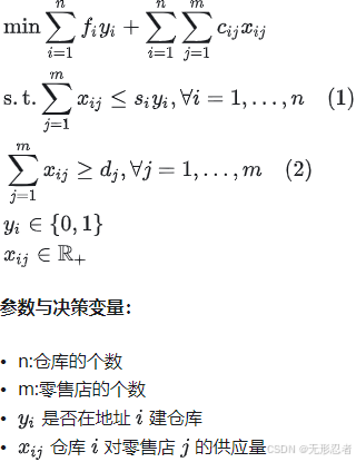
2.1问题描述

2.2选址问题的原始MIP模型

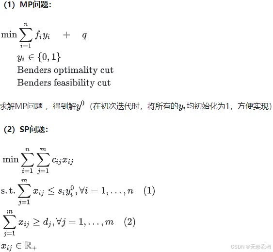
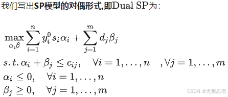
2.3将原始MIP模型进行分解

(3)更新MP问题

根据Benders算法流程，我们向MP问题中添加Benders optimality cut和Benders feasibility cut，Benders主问题可以写为：

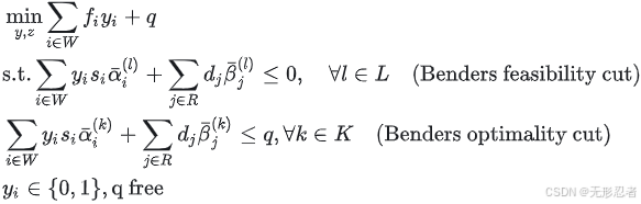
其中，K是子问题的对偶问题Dual SP的极点(extreme point，其实就是最优解)的集合

L是子问题的对偶问题Dual SP的极射线(extreme ray，其实就是无界射线)的集合

3.python调用gurobi实现Benders Decomposition求解FLP（Facility Location Problem）

核心代码：

import numpy as np
from gurobipy import *from principle.input_data import InputDataclass Subproblem:def __init__(self, data, Q, E):self.data = dataself.sub_problem = Model("sub_problem")self.sub_problem.setParam('InfUnbdInfo', 1)self.alpha = self.sub_problem.addVars([i for i in range(self.data['w_size'])],lb= -np.inf,ub= 0, name="alpha")  # 资源约束的对偶变量self.beta = self.sub_problem.addVars([j for j in range(self.data['r_size'])],lb= 0,ub= np.inf, name="beta")  # 需求约束的对偶变量self.Q = Qself.E = Eself.subCon = [['' for _ in range(self.data['r_size'])] for _ in range(self.data['w_size'])]def add_constrs(self):# 子问题对偶问题添加约束for i in range(self.data['w_size']):for j in range(self.data['r_size']):self.subCon[i][j] = self.sub_problem.addConstr(self.alpha[i] + self.beta[j] <= self.data['c'][i][j])def set_objective(self, bar_y):# 子问题对偶问题的目标函数self.sub_problem.setObjective(quicksum(bar_y[i] * self.data['supply'][i] * self.alpha[i] for i in range(self.data['w_size'])) +quicksum(self.data['demand'][j] * self.beta[j] for j in range(self.data['r_size'])), GRB.MAXIMIZE)def solve(self):self.sub_problem.optimize()def get_status(self, iter_i):if self.sub_problem.status == GRB.UNBOUNDED:# feasible cutitem = dict()item["alpha"] = {i: self.alpha[i].unbdRay for i in range(self.data['w_size'])}item["beta"] = {j: self.beta[j].unbdRay for j in range(self.data['r_size'])}self.Q[iter_i] = itemelif self.sub_problem.status == GRB.OPTIMAL:# optimality cutitem = dict()item["alpha"] = {i: self.alpha[i].x for i in range(self.data['w_size'])}item["beta"] = {j: self.beta[j].x for j in range(self.data['r_size'])}self.E[iter_i] = itemreturn self.sub_problem.statusdef get_objval(self):return self.sub_problem.objVal if self.sub_problem.status == GRB.OPTIMAL else -np.infdef write(self, sub_name):self.sub_problem.write(sub_name + ".lp")def get_solution(self):# duals = self.sub_problem.getAttr("Pi", self.sub_problem.getConstrs())# for con in self.sub_problem.getConstrs():  # 循环获取#     if con.Pi > 0.1 :#         print(con.ConstrName, '----', con.Pi)# 处理对偶变量的值for i in range(self.data['w_size']):for j in range(self.data['r_size']):dual_var = self.sub_problem.getConstrByName(self.subCon[i][j].constrName).Piif dual_var > 0.01:print("ship ["+ str(i) +"] to ["+ str(j) +"]"+ str(dual_var))class Master:def __init__(self, data, Q, E):self.data = dataself.master_problem = Model("master_problem")# 决策变量初始化self.y = self.master_problem.addVars([i for i in range(self.data['w_size'])], vtype=GRB.BINARY, name="y")# 参数约束 子问题中的目标值，对应松弛的主问题模型中qself.q = self.master_problem.addVar(vtype=GRB.CONTINUOUS, name="q")self.Q = Qself.E = Edef add_optimality_cut(self, iter_i):# general benders optimality cutfor item in self.E.values():self.master_problem.addConstr(quicksum(self.y[i] * self.data['supply'][i] * item["alpha"][i] for i in range(self.data['w_size'])) +quicksum(self.data['demand'][j] * item["beta"][j] for j in range(self.data['r_size']))<= self.q, name = "optimality_cut_" + str(iter_i))def add_feasiblity_cut(self, iter_i):# benders feasiblity cutfor item in self.Q.values():self.master_problem.addConstr(quicksum(self.y[i] * self.data['supply'][i] * item["alpha"][i] for i in range(self.data['w_size'])) +quicksum(self.data['demand'][j] * item["beta"][j] for j in range(self.data['r_size']))<= 0, name = "feasiblity_cut_" + str(iter_i))def set_objective(self):# 主问题建模self.master_problem.setObjective(quicksum(self.data['fixed_c'][i] * self.y[i] for i in range(self.data['w_size'])) + self.q, GRB.MINIMIZE)def solve(self):self.master_problem.optimize()def get_solution(self):bar_y = dict()for i in range(self.data['w_size']):bar_y[i] = 1 if self.y[i].x > 0.01 else 0return bar_ydef get_objval(self):return self.master_problem.objVal if self.master_problem.status == GRB.OPTIMAL else -np.infdef write(self, name):self.master_problem.write(name + ".lp")

4.算例与求解结果

import numpy as npclass InputData:@staticmethoddef read_data():data = dict()data['w_size'] = 25data['r_size'] = 6data['supply'] = [23070,18290,20010,15080,17540,21090,16650,18420,19160,18860,22690,19360,22330,15440,19330,17110,15380,18690,20720,21220,16720,21540,16500,15310,18970]data['demand'] = [12000, 12000, 14000, 13500, 25000, 29000]data['fixed_c'] = [500000,500000,500000,500000,500000,500000,500000,500000,500000,500000,500000,500000,500000,500000,500000,500000,500000,500000,500000,500000,500000,500000,500000,500000,500000]data['c'] = [[73.78, 14.76,86.82, 91.19,51.03, 76.49],[60.28, 20.92,76.43, 83.99,58.84, 68.86],[58.18, 21.64,69.84, 72.39,61.64, 58.39],[50.37, 21.74,61.49, 65.72,60.48, 56.68],[42.73, 35.19,44.11, 58.08,65.76, 55.51],[44.62, 39.21,44.44, 48.32,76.12, 51.17],[49.31, 51.72,36.27, 42.96,84.52, 49.61],[50.79, 59.25,22.53, 33.22,94.30, 49.66],[51.93, 72.13,21.66, 29.39,93.52, 49.63],[65.90, 13.07,79.59, 86.07,46.83, 69.55],[50.79,  9.99,67.83, 78.81,49.34, 60.79],[47.51, 12.95,59.57, 67.71,51.13, 54.65],[39.36, 19.01,56.39, 62.37,57.25, 47.91],[33.55, 30.16,40.66, 48.50,60.83, 42.51],[34.17, 40.46,40.23, 47.10,66.22, 38.94],[41.68, 53.03,22.56, 30.89,77.22, 35.88],[42.75, 62.94,18.58, 27.02,80.36, 40.11],[46.46, 71.17,17.17, 21.16,91.65, 41.56],[56.83,  8.84,83.99, 91.88,41.38, 67.79],[46.21,  2.92,68.94, 76.86,38.89, 60.38],[41.67, 11.69,61.05, 70.06,43.24, 48.48],[25.57, 17.59,54.93, 57.07,44.93, 43.97],[28.16, 29.39,38.64, 46.48,50.16, 34.20],[26.97, 41.62,29.72, 40.61,59.56, 31.21],[34.24, 54.09,22.13, 28.43,69.68, 24.09]]return data

算法迭代的日志展示如下：

====================================================================================================
iteration at 9
Gurobi Optimizer version 11.0.2 build v11.0.2rc0 (win64 - Windows 10.0 (19045.2))CPU model: Intel(R) Core(TM) i7-8700 CPU @ 3.20GHz, instruction set [SSE2|AVX|AVX2]
Thread count: 6 physical cores, 12 logical processors, using up to 12 threadsOptimize a model with 150 rows, 31 columns and 300 nonzeros
Coefficient statistics:Matrix range     [1e+00, 1e+00]Objective range  [1e+04, 3e+04]Bounds range     [0e+00, 0e+00]RHS range        [3e+00, 9e+01]
LP warm-start: use basis
Iteration    Objective       Primal Inf.    Dual Inf.      Time0    4.6710000e+34   8.100000e+31   4.671000e+04      0s35    2.7352069e+06   0.000000e+00   0.000000e+00      0sSolved in 35 iterations and 0.00 seconds (0.00 work units)
Optimal objective  2.735206900e+06
ship [16] to [2]8810.0
ship [16] to [5]960.0
ship [17] to [2]5190.0
ship [17] to [3]13500.0
ship [19] to [1]12000.0
ship [19] to [4]9220.0
ship [21] to [0]5760.0
ship [21] to [4]15780.0
ship [23] to [0]6240.0
ship [23] to [5]9070.0
ship [24] to [5]18970.0
Q  1
E  9
y:
{0: 0, 1: 0, 2: 0, 3: 0, 4: 0, 5: 0, 6: 0, 7: 0, 8: 0, 9: 0, 10: 0, 11: 0, 12: 0, 13: 0, 14: 0, 15: 0, 16: 1, 17: 1, 18: 0, 19: 1, 20: 0, 21: 1, 22: 0, 23: 1, 24: 1}
Gurobi Optimizer version 11.0.2 build v11.0.2rc0 (win64 - Windows 10.0 (19045.2))CPU model: Intel(R) Core(TM) i7-8700 CPU @ 3.20GHz, instruction set [SSE2|AVX|AVX2]
Thread count: 6 physical cores, 12 logical processors, using up to 12 threadsOptimize a model with 46 rows, 26 columns and 715 nonzeros
Model fingerprint: 0xd3a9408a
Variable types: 1 continuous, 25 integer (25 binary)
Coefficient statistics:Matrix range     [1e+00, 1e+06]Objective range  [1e+00, 5e+05]Bounds range     [1e+00, 1e+00]RHS range        [1e+05, 6e+06]MIP start from previous solve produced solution with objective 5.73521e+06 (0.00s)
Loaded MIP start from previous solve with objective 5.73521e+06Presolve removed 36 rows and 0 columns
Presolve time: 0.00s
Presolved: 10 rows, 26 columns, 164 nonzeros
Variable types: 1 continuous, 25 integer (25 binary)Root relaxation: objective 5.391367e+06, 11 iterations, 0.00 seconds (0.00 work units)Nodes    |    Current Node    |     Objective Bounds      |     WorkExpl Unexpl |  Obj  Depth IntInf | Incumbent    BestBd   Gap | It/Node Time0     0 5391366.52    0    4 5735206.90 5391366.52  6.00%     -    0s
H    0     0                    5700871.8000 5391366.52  5.43%     -    0s
H    0     0                    5675356.0000 5422912.77  4.45%     -    0s0     0 5426773.19    0    7 5675356.00 5426773.19  4.38%     -    0s
H    0     0                    5667218.1000 5433392.41  4.13%     -    0s0     0 5441823.56    0    6 5667218.10 5441823.56  3.98%     -    0s0     0 5459350.96    0    6 5667218.10 5459350.96  3.67%     -    0s0     0 5481319.95    0    6 5667218.10 5481319.95  3.28%     -    0s
H    0     0                    5661907.9000 5481319.95  3.19%     -    0s0     0 5501705.15    0    8 5661907.90 5501705.15  2.83%     -    0s0     0 5501705.15    0    9 5661907.90 5501705.15  2.83%     -    0s0     0 5510139.70    0    8 5661907.90 5510139.70  2.68%     -    0s0     0 5510139.70    0    9 5661907.90 5510139.70  2.68%     -    0s0     0 5510139.70    0    9 5661907.90 5510139.70  2.68%     -    0s0     0 5510139.70    0    8 5661907.90 5510139.70  2.68%     -    0s0     0 5510139.70    0    7 5661907.90 5510139.70  2.68%     -    0s0     0 5510340.64    0    8 5661907.90 5510340.64  2.68%     -    0s0     2 5515530.88    0    8 5661907.90 5515530.88  2.59%     -    0sCutting planes:Gomory: 1Lift-and-project: 1Cover: 3MIR: 7Explored 97 nodes (445 simplex iterations) in 0.03 seconds (0.01 work units)
Thread count was 12 (of 12 available processors)Solution count 5: 5.66191e+06 5.66722e+06 5.67536e+06 ... 5.73521e+06Optimal solution found (tolerance 1.00e-04)
Best objective 5.661907900000e+06, best bound 5.661907900000e+06, gap 0.0000%
Warning: linear constraint 2 and linear constraint 3 have the same name "optimality_cut_2"
ub:5735206.9
lb:5661907.9

最优解信息：

ship [16] to [2]8810.0
ship [16] to [5]960.0
ship [17] to [2]5190.0
ship [17] to [3]13500.0
ship [19] to [1]12000.0
ship [19] to [4]9220.0
ship [21] to [0]5760.0
ship [21] to [4]15780.0
ship [23] to [0]6240.0
ship [23] to [5]9070.0
ship [24] to [5]18970.0
y:
{0: 0, 1: 0, 2: 0, 3: 0, 4: 0, 5: 0, 6: 0, 7: 0, 8: 0, 9: 0, 10: 0, 11: 0, 12: 0, 13: 0, 14: 0, 15: 0, 16: 1, 17: 1, 18: 0, 19: 1, 20: 0, 21: 1, 22: 0, 23: 1, 24: 1}
ub:5735206.9