Cost Function for Logistic Regression
- 1. 平方差能否用于逻辑回归?
- 2. 逻辑损失函数loss
- 3. 损失函数cost
- 附录
导入所需的库
import numpy as np
%matplotlib widget
import matplotlib.pyplot as plt
from plt_logistic_loss import  plt_logistic_cost, plt_two_logistic_loss_curves, plt_simple_example
from plt_logistic_loss import soup_bowl, plt_logistic_squared_error
from lab_utils_common import  plot_data, sigmoid, dlc
plt.style.use('./deeplearning.mplstyle')
1. 平方差能否用于逻辑回归?
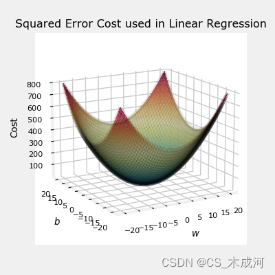
在前面的线性回归中,我们使用的是 squared error cost function,带有一个变量的squared error cost 为:
J ( w , b ) = 1 2 m ∑ i = 0 m − 1 ( f w , b ( x ( i ) ) − y ( i ) ) 2 (1) J(w,b) = \frac{1}{2m} \sum\limits_{i = 0}^{m-1} (f_{w,b}(x^{(i)}) - y^{(i)})^2 \tag{1} J(w,b)=2m1i=0∑m−1(fw,b(x(i))−y(i))2(1)
其中,
f w , b ( x ( i ) ) = w x ( i ) + b (2) f_{w,b}(x^{(i)}) = wx^{(i)} + b \tag{2} fw,b(x(i))=wx(i)+b(2)
squared error cost有一个很好的性质,就是对cost求导会得到最小值。
soup_bowl()
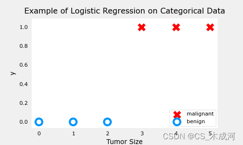
这个cost函数在线性回归中表现得很好,当然,它也适用于逻辑回归。然而, f w b ( x ) f_{wb}(x) fwb(x)现在有一个非线性的部分,即sigmoid函数: f w , b ( x ( i ) ) = s i g m o i d ( w x ( i ) + b ) f_{w,b}(x^{(i)}) = sigmoid(wx^{(i)} + b ) fw,b(x(i))=sigmoid(wx(i)+b)。接下来,我们尝试使用squared error cost在以前博客的样例中,此时包括sigmod。
训练数据:
x_train = np.array([0., 1, 2, 3, 4, 5],dtype=np.longdouble)
y_train = np.array([0,  0, 0, 1, 1, 1],dtype=np.longdouble)
plt_simple_example(x_train, y_train)
现在,用squared error cost 绘制cost的曲面图:
J ( w , b ) = 1 2 m ∑ i = 0 m − 1 ( f w , b ( x ( i ) ) − y ( i ) ) 2 J(w,b) = \frac{1}{2m} \sum\limits_{i = 0}^{m-1} (f_{w,b}(x^{(i)}) - y^{(i)})^2 J(w,b)=2m1i=0∑m−1(fw,b(x(i))−y(i))2
其中,
f w , b ( x ( i ) ) = s i g m o i d ( w x ( i ) + b ) f_{w,b}(x^{(i)}) = sigmoid(wx^{(i)} + b ) fw,b(x(i))=sigmoid(wx(i)+b)
plt.close('all')
plt_logistic_squared_error(x_train,y_train)
plt.show()
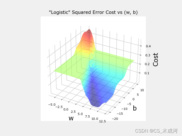
虽然这产生了一个非常有趣的曲面图,但上面的曲面并不像线性回归的“汤碗”那么光滑。逻辑回归需要一个更适合其非线性性质的cost函数。
2. 逻辑损失函数loss
逻辑回归使用更适合分类任务的Loss函数,其中目标是0或1而不是任何数字。
注意:Loss是单个示例与其目标值之差的度量,而Cost是训练集上损失的度量。
定义: l o s s ( f w , b ( x ( i ) ) , y ( i ) ) loss(f_{\mathbf{w},b}(\mathbf{x}^{(i)}), y^{(i)}) loss(fw,b(x(i)),y(i)) 是单个数据点的cost:
l o s s ( f w , b ( x ( i ) ) , y ( i ) ) = { − log ( f w , b ( x ( i ) ) ) if y ( i ) = 1 log ( 1 − f w , b ( x ( i ) ) ) if y ( i ) = 0 \begin{equation} loss(f_{\mathbf{w},b}(\mathbf{x}^{(i)}), y^{(i)}) = \begin{cases} - \log\left(f_{\mathbf{w},b}\left( \mathbf{x}^{(i)} \right) \right) & \text{if $y^{(i)}=1$}\\ \log \left( 1 - f_{\mathbf{w},b}\left( \mathbf{x}^{(i)} \right) \right) & \text{if $y^{(i)}=0$} \end{cases} \end{equation} loss(fw,b(x(i)),y(i))={−log(fw,b(x(i)))log(1−fw,b(x(i)))if y(i)=1if y(i)=0
f w , b ( x ( i ) ) f_{\mathbf{w},b}(\mathbf{x}^{(i)}) fw,b(x(i)) 是模型的预测值, y ( i ) y^{(i)} y(i) 是目标值.
f w , b ( x ( i ) ) = g ( w ⋅ x ( i ) + b ) f_{\mathbf{w},b}(\mathbf{x}^{(i)}) = g(\mathbf{w} \cdot\mathbf{x}^{(i)}+b) fw,b(x(i))=g(w⋅x(i)+b) ,其中 g g g 是 sigmoid 函数.
这个损失函数的定义特点在于使用了两条不同的曲线。一个用于目标为0或( y = 0 y=0 y=0)的情况,另一个用于目标为1 ( y = 1 y=1 y=1)的情况。这些曲线结合起来为损失函数提供了帮助,即当预测与目标匹配时为零,当预测与目标不同时 l o s s loss loss 值迅速增加。
plt_two_logistic_loss_curves()
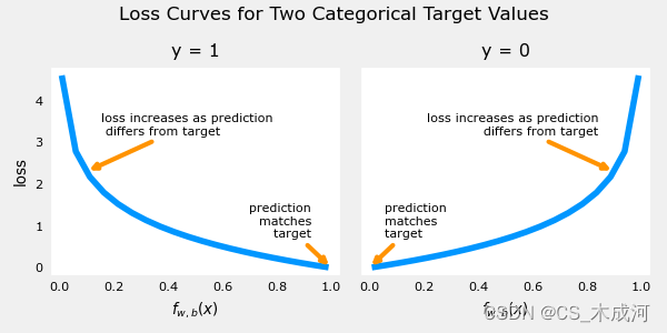
综合起来,曲线类似于平方差损失的二次曲线。注意,x轴是 f w , b f_{\mathbf{w},b} fw,b,是sigmoid的输出。sigmoid 输出严格在0到1之间。
上面的损失函数可以简写为:
l o s s ( f w , b ( x ( i ) ) , y ( i ) ) = ( − y ( i ) log ( f w , b ( x ( i ) ) ) − ( 1 − y ( i ) ) log ( 1 − f w , b ( x ( i ) ) ) loss(f_{\mathbf{w},b}(\mathbf{x}^{(i)}), y^{(i)}) = (-y^{(i)} \log\left(f_{\mathbf{w},b}\left( \mathbf{x}^{(i)} \right) \right) - \left( 1 - y^{(i)}\right) \log \left( 1 - f_{\mathbf{w},b}\left( \mathbf{x}^{(i)} \right) \right) loss(fw,b(x(i)),y(i))=(−y(i)log(fw,b(x(i)))−(1−y(i))log(1−fw,b(x(i)))
可以将方程分成两部分:
当 y ( i ) = 0 y^{(i)} = 0 y(i)=0 时,左边的项被消除:
l o s s ( f w , b ( x ( i ) ) , 0 ) = ( − ( 0 ) log ( f w , b ( x ( i ) ) ) − ( 1 − 0 ) log ( 1 − f w , b ( x ( i ) ) ) = − log ( 1 − f w , b ( x ( i ) ) ) \begin{align} loss(f_{\mathbf{w},b}(\mathbf{x}^{(i)}), 0) &= (-(0) \log\left(f_{\mathbf{w},b}\left( \mathbf{x}^{(i)} \right) \right) - \left( 1 - 0\right) \log \left( 1 - f_{\mathbf{w},b}\left( \mathbf{x}^{(i)} \right) \right) \\ &= -\log \left( 1 - f_{\mathbf{w},b}\left( \mathbf{x}^{(i)} \right) \right) \end{align} loss(fw,b(x(i)),0)=(−(0)log(fw,b(x(i)))−(1−0)log(1−fw,b(x(i)))=−log(1−fw,b(x(i)))
当 y ( i ) = 1 y^{(i)} = 1 y(i)=1 时, 右边的项被消除:
l o s s ( f w , b ( x ( i ) ) , 1 ) = ( − ( 1 ) log ( f w , b ( x ( i ) ) ) − ( 1 − 1 ) log ( 1 − f w , b ( x ( i ) ) ) = − log ( f w , b ( x ( i ) ) ) \begin{align} loss(f_{\mathbf{w},b}(\mathbf{x}^{(i)}), 1) &= (-(1) \log\left(f_{\mathbf{w},b}\left( \mathbf{x}^{(i)} \right) \right) - \left( 1 - 1\right) \log \left( 1 - f_{\mathbf{w},b}\left( \mathbf{x}^{(i)} \right) \right)\\ &= -\log\left(f_{\mathbf{w},b}\left( \mathbf{x}^{(i)} \right) \right) \end{align} loss(fw,b(x(i)),1)=(−(1)log(fw,b(x(i)))−(1−1)log(1−fw,b(x(i)))=−log(fw,b(x(i)))
所以,我们可以通过这个新的逻辑损失函数得到一个包含所有样例的损失函数。
上面示例的损失与参数曲线为:
plt.close('all')
cst = plt_logistic_cost(x_train,y_train)
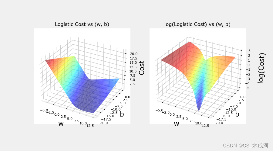
这条曲线非常适合梯度下降。它没有局部极小值或不连续点。需要注意的是,它不像平方差损失那样呈现“碗”状。绘制cost和log cost来说明,当cost较小时,曲线有一个斜率并继续下降。
3. 损失函数cost
导入数据集
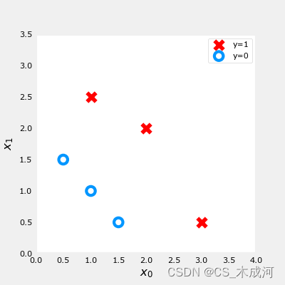
X_train = np.array([[0.5, 1.5], [1,1], [1.5, 0.5], [3, 0.5], [2, 2], [1, 2.5]])  #(m,n)
y_train = np.array([0, 0, 0, 1, 1, 1])                                           #(m,)
训练数据绘图可视化:
fig,ax = plt.subplots(1,1,figsize=(4,4))
plot_data(X_train, y_train, ax)# Set both axes to be from 0-4
ax.axis([0, 4, 0, 3.5])
ax.set_ylabel('$x_1$', fontsize=12)
ax.set_xlabel('$x_0$', fontsize=12)
plt.show()
前面介绍了一个样例的逻辑 loss 函数,这里我们根据 loss 计算包括所有样例的cost 。
对于逻辑回归,cost 函数表示为:
J ( w , b ) = 1 m ∑ i = 0 m − 1 [ l o s s ( f w , b ( x ( i ) ) , y ( i ) ) ] (1) J(\mathbf{w},b) = \frac{1}{m} \sum_{i=0}^{m-1} \left[ loss(f_{\mathbf{w},b}(\mathbf{x}^{(i)}), y^{(i)}) \right] \tag{1} J(w,b)=m1i=0∑m−1[loss(fw,b(x(i)),y(i))](1)
其中,
- l o s s ( f w , b ( x ( i ) ) , y ( i ) ) loss(f_{\mathbf{w},b}(\mathbf{x}^{(i)}), y^{(i)}) loss(fw,b(x(i)),y(i)) 是一个单独数据点的cost,即:
l o s s ( f w , b ( x ( i ) ) , y ( i ) ) = − y ( i ) log ( f w , b ( x ( i ) ) ) − ( 1 − y ( i ) ) log ( 1 − f w , b ( x ( i ) ) ) (2) loss(f_{\mathbf{w},b}(\mathbf{x}^{(i)}), y^{(i)}) = -y^{(i)} \log\left(f_{\mathbf{w},b}\left( \mathbf{x}^{(i)} \right) \right) - \left( 1 - y^{(i)}\right) \log \left( 1 - f_{\mathbf{w},b}\left( \mathbf{x}^{(i)} \right) \right) \tag{2} loss(fw,b(x(i)),y(i))=−y(i)log(fw,b(x(i)))−(1−y(i))log(1−fw,b(x(i)))(2)
其中,m是数据集中训练样例的数量。
f w , b ( x ( i ) ) = g ( z ( i ) ) z ( i ) = w ⋅ x ( i ) + b g ( z ( i ) ) = 1 1 + e − z ( i ) \begin{align} f_{\mathbf{w},b}(\mathbf{x^{(i)}}) &= g(z^{(i)})\tag{3} \\ z^{(i)} &= \mathbf{w} \cdot \mathbf{x}^{(i)}+ b\tag{4} \\ g(z^{(i)}) &= \frac{1}{1+e^{-z^{(i)}}}\tag{5} \end{align} fw,b(x(i))z(i)g(z(i))=g(z(i))=w⋅x(i)+b=1+e−z(i)1(3)(4)(5)
其代码描述为:
compute_cost_logistic算法在所有的样例上循环,计算每个样例的损失并相加。
变量 X 和 y 不是标量,而是shape分别为( m , n m, n m,n) 和 ( m m m) 的矩阵。其中 n n n 是特征的数量, m m m 是训练样例的数量.
def compute_cost_logistic(X, y, w, b):"""Computes costArgs:X (ndarray (m,n)): Data, m examples with n featuresy (ndarray (m,)) : target valuesw (ndarray (n,)) : model parameters b (scalar) : model parameterReturns:cost (scalar): cost"""m = X.shape[0]cost = 0.0for i in range(m):z_i = np.dot(X[i],w) + bf_wb_i = sigmoid(z_i)cost += -y[i]*np.log(f_wb_i) - (1-y[i])*np.log(1-f_wb_i)cost = cost / mreturn cost
测试一下:
w_tmp = np.array([1,1])
b_tmp = -3
print(compute_cost_logistic(X_train, y_train, w_tmp, b_tmp))
输出为:0.3668667864055175
附录
lab_utils_common.py 源码:
"""
lab_utils_commoncontains common routines and variable definitionsused by all the labs in this week.by contrast, specific, large plotting routines will be in separate filesand are generally imported into the week where they are used.those files will import this file
"""
import copy
import math
import numpy as np
import matplotlib.pyplot as plt
from matplotlib.patches import FancyArrowPatch
from ipywidgets import Outputnp.set_printoptions(precision=2)dlc = dict(dlblue = '#0096ff', dlorange = '#FF9300', dldarkred='#C00000', dlmagenta='#FF40FF', dlpurple='#7030A0')
dlblue = '#0096ff'; dlorange = '#FF9300'; dldarkred='#C00000'; dlmagenta='#FF40FF'; dlpurple='#7030A0'
dlcolors = [dlblue, dlorange, dldarkred, dlmagenta, dlpurple]
plt.style.use('./deeplearning.mplstyle')def sigmoid(z):"""Compute the sigmoid of zParameters----------z : array_likeA scalar or numpy array of any size.Returns-------g : array_likesigmoid(z)"""z = np.clip( z, -500, 500 )           # protect against overflowg = 1.0/(1.0+np.exp(-z))return g##########################################################
# Regression Routines
##########################################################def predict_logistic(X, w, b):""" performs prediction """return sigmoid(X @ w + b)def predict_linear(X, w, b):""" performs prediction """return X @ w + bdef compute_cost_logistic(X, y, w, b, lambda_=0, safe=False):"""Computes cost using logistic loss, non-matrix versionArgs:X (ndarray): Shape (m,n)  matrix of examples with n featuresy (ndarray): Shape (m,)   target valuesw (ndarray): Shape (n,)   parameters for predictionb (scalar):               parameter  for predictionlambda_ : (scalar, float) Controls amount of regularization, 0 = no regularizationsafe : (boolean)          True-selects under/overflow safe algorithmReturns:cost (scalar): cost"""m,n = X.shapecost = 0.0for i in range(m):z_i    = np.dot(X[i],w) + b                                             #(n,)(n,) or (n,) ()if safe:  #avoids overflowscost += -(y[i] * z_i ) + log_1pexp(z_i)else:f_wb_i = sigmoid(z_i)                                                   #(n,)cost  += -y[i] * np.log(f_wb_i) - (1 - y[i]) * np.log(1 - f_wb_i)       # scalarcost = cost/mreg_cost = 0if lambda_ != 0:for j in range(n):reg_cost += (w[j]**2)                                               # scalarreg_cost = (lambda_/(2*m))*reg_costreturn cost + reg_costdef log_1pexp(x, maximum=20):''' approximate log(1+exp^x)https://stats.stackexchange.com/questions/475589/numerical-computation-of-cross-entropy-in-practiceArgs:x   : (ndarray Shape (n,1) or (n,)  inputout : (ndarray Shape matches x      output ~= np.log(1+exp(x))'''out  = np.zeros_like(x,dtype=float)i    = x <= maximumni   = np.logical_not(i)out[i]  = np.log(1 + np.exp(x[i]))out[ni] = x[ni]return outdef compute_cost_matrix(X, y, w, b, logistic=False, lambda_=0, safe=True):"""Computes the cost using  using matricesArgs:X : (ndarray, Shape (m,n))          matrix of examplesy : (ndarray  Shape (m,) or (m,1))  target value of each examplew : (ndarray  Shape (n,) or (n,1))  Values of parameter(s) of the modelb : (scalar )                       Values of parameter of the modelverbose : (Boolean) If true, print out intermediate value f_wbReturns:total_cost: (scalar)                cost"""m = X.shape[0]y = y.reshape(-1,1)             # ensure 2Dw = w.reshape(-1,1)             # ensure 2Dif logistic:if safe:  #safe from overflowz = X @ w + b                                                           #(m,n)(n,1)=(m,1)cost = -(y * z) + log_1pexp(z)cost = np.sum(cost)/m                                                   # (scalar)else:f    = sigmoid(X @ w + b)                                               # (m,n)(n,1) = (m,1)cost = (1/m)*(np.dot(-y.T, np.log(f)) - np.dot((1-y).T, np.log(1-f)))   # (1,m)(m,1) = (1,1)cost = cost[0,0]                                                        # scalarelse:f    = X @ w + b                                                        # (m,n)(n,1) = (m,1)cost = (1/(2*m)) * np.sum((f - y)**2)                                   # scalarreg_cost = (lambda_/(2*m)) * np.sum(w**2)                                   # scalartotal_cost = cost + reg_cost                                                # scalarreturn total_cost                                                           # scalardef compute_gradient_matrix(X, y, w, b, logistic=False, lambda_=0):"""Computes the gradient using matricesArgs:X : (ndarray, Shape (m,n))          matrix of examplesy : (ndarray  Shape (m,) or (m,1))  target value of each examplew : (ndarray  Shape (n,) or (n,1))  Values of parameters of the modelb : (scalar )                       Values of parameter of the modellogistic: (boolean)                 linear if false, logistic if truelambda_:  (float)                   applies regularization if non-zeroReturnsdj_dw: (array_like Shape (n,1))     The gradient of the cost w.r.t. the parameters wdj_db: (scalar)                     The gradient of the cost w.r.t. the parameter b"""m = X.shape[0]y = y.reshape(-1,1)             # ensure 2Dw = w.reshape(-1,1)             # ensure 2Df_wb  = sigmoid( X @ w + b ) if logistic else  X @ w + b      # (m,n)(n,1) = (m,1)err   = f_wb - y                                              # (m,1)dj_dw = (1/m) * (X.T @ err)                                   # (n,m)(m,1) = (n,1)dj_db = (1/m) * np.sum(err)                                   # scalardj_dw += (lambda_/m) * w        # regularize                  # (n,1)return dj_db, dj_dw                                           # scalar, (n,1)def gradient_descent(X, y, w_in, b_in, alpha, num_iters, logistic=False, lambda_=0, verbose=True):"""Performs batch gradient descent to learn theta. Updates theta by takingnum_iters gradient steps with learning rate alphaArgs:X (ndarray):    Shape (m,n)         matrix of examplesy (ndarray):    Shape (m,) or (m,1) target value of each examplew_in (ndarray): Shape (n,) or (n,1) Initial values of parameters of the modelb_in (scalar):                      Initial value of parameter of the modellogistic: (boolean)                 linear if false, logistic if truelambda_:  (float)                   applies regularization if non-zeroalpha (float):                      Learning ratenum_iters (int):                    number of iterations to run gradient descentReturns:w (ndarray): Shape (n,) or (n,1)    Updated values of parameters; matches incoming shapeb (scalar):                         Updated value of parameter"""# An array to store cost J and w's at each iteration primarily for graphing laterJ_history = []w = copy.deepcopy(w_in)  #avoid modifying global w within functionb = b_inw = w.reshape(-1,1)      #prep for matrix operationsy = y.reshape(-1,1)for i in range(num_iters):# Calculate the gradient and update the parametersdj_db,dj_dw = compute_gradient_matrix(X, y, w, b, logistic, lambda_)# Update Parameters using w, b, alpha and gradientw = w - alpha * dj_dwb = b - alpha * dj_db# Save cost J at each iterationif i<100000:      # prevent resource exhaustionJ_history.append( compute_cost_matrix(X, y, w, b, logistic, lambda_) )# Print cost every at intervals 10 times or as many iterations if < 10if i% math.ceil(num_iters / 10) == 0:if verbose: print(f"Iteration {i:4d}: Cost {J_history[-1]}   ")return w.reshape(w_in.shape), b, J_history  #return final w,b and J history for graphingdef zscore_normalize_features(X):"""computes  X, zcore normalized by columnArgs:X (ndarray): Shape (m,n) input data, m examples, n featuresReturns:X_norm (ndarray): Shape (m,n)  input normalized by columnmu (ndarray):     Shape (n,)   mean of each featuresigma (ndarray):  Shape (n,)   standard deviation of each feature"""# find the mean of each column/featuremu     = np.mean(X, axis=0)                 # mu will have shape (n,)# find the standard deviation of each column/featuresigma  = np.std(X, axis=0)                  # sigma will have shape (n,)# element-wise, subtract mu for that column from each example, divide by std for that columnX_norm = (X - mu) / sigmareturn X_norm, mu, sigma#check our work
#from sklearn.preprocessing import scale
#scale(X_orig, axis=0, with_mean=True, with_std=True, copy=True)######################################################
# Common Plotting Routines
######################################################def plot_data(X, y, ax, pos_label="y=1", neg_label="y=0", s=80, loc='best' ):""" plots logistic data with two axis """# Find Indices of Positive and Negative Examplespos = y == 1neg = y == 0pos = pos.reshape(-1,)  #work with 1D or 1D y vectorsneg = neg.reshape(-1,)# Plot examplesax.scatter(X[pos, 0], X[pos, 1], marker='x', s=s, c = 'red', label=pos_label)ax.scatter(X[neg, 0], X[neg, 1], marker='o', s=s, label=neg_label, facecolors='none', edgecolors=dlblue, lw=3)ax.legend(loc=loc)ax.figure.canvas.toolbar_visible = Falseax.figure.canvas.header_visible = Falseax.figure.canvas.footer_visible = Falsedef plt_tumor_data(x, y, ax):""" plots tumor data on one axis """pos = y == 1neg = y == 0ax.scatter(x[pos], y[pos], marker='x', s=80, c = 'red', label="malignant")ax.scatter(x[neg], y[neg], marker='o', s=100, label="benign", facecolors='none', edgecolors=dlblue,lw=3)ax.set_ylim(-0.175,1.1)ax.set_ylabel('y')ax.set_xlabel('Tumor Size')ax.set_title("Logistic Regression on Categorical Data")ax.figure.canvas.toolbar_visible = Falseax.figure.canvas.header_visible = Falseax.figure.canvas.footer_visible = False# Draws a threshold at 0.5
def draw_vthresh(ax,x):""" draws a threshold """ylim = ax.get_ylim()xlim = ax.get_xlim()ax.fill_between([xlim[0], x], [ylim[1], ylim[1]], alpha=0.2, color=dlblue)ax.fill_between([x, xlim[1]], [ylim[1], ylim[1]], alpha=0.2, color=dldarkred)ax.annotate("z >= 0", xy= [x,0.5], xycoords='data',xytext=[30,5],textcoords='offset points')d = FancyArrowPatch(posA=(x, 0.5), posB=(x+3, 0.5), color=dldarkred,arrowstyle='simple, head_width=5, head_length=10, tail_width=0.0',)ax.add_artist(d)ax.annotate("z < 0", xy= [x,0.5], xycoords='data',xytext=[-50,5],textcoords='offset points', ha='left')f = FancyArrowPatch(posA=(x, 0.5), posB=(x-3, 0.5), color=dlblue,arrowstyle='simple, head_width=5, head_length=10, tail_width=0.0',)ax.add_artist(f)
plt_logistic_loss.py 源码:
"""----------------------------------------------------------------logistic_loss plotting routines and support
"""from matplotlib import cm
from lab_utils_common import sigmoid, dlblue, dlorange, np, plt, compute_cost_matrixdef compute_cost_logistic_sq_err(X, y, w, b):"""compute sq error cost on logicist data (for negative example only, not used in practice)Args:X (ndarray): Shape (m,n) matrix of examples with multiple featuresw (ndarray): Shape (n)   parameters for predictionb (scalar):              parameter  for predictionReturns:cost (scalar): cost"""m = X.shape[0]cost = 0.0for i in range(m):z_i = np.dot(X[i],w) + bf_wb_i = sigmoid(z_i)                 #add sigmoid to normal sq error cost for linear regressioncost = cost + (f_wb_i - y[i])**2cost = cost / (2 * m)return np.squeeze(cost)def plt_logistic_squared_error(X,y):""" plots logistic squared error for demonstration """wx, by = np.meshgrid(np.linspace(-6,12,50),np.linspace(10, -20, 40))points = np.c_[wx.ravel(), by.ravel()]cost = np.zeros(points.shape[0])for i in range(points.shape[0]):w,b = points[i]cost[i] = compute_cost_logistic_sq_err(X.reshape(-1,1), y, w, b)cost = cost.reshape(wx.shape)fig = plt.figure()fig.canvas.toolbar_visible = Falsefig.canvas.header_visible = Falsefig.canvas.footer_visible = Falseax = fig.add_subplot(1, 1, 1, projection='3d')ax.plot_surface(wx, by, cost, alpha=0.6,cmap=cm.jet,)ax.set_xlabel('w', fontsize=16)ax.set_ylabel('b', fontsize=16)ax.set_zlabel("Cost", rotation=90, fontsize=16)ax.set_title('"Logistic" Squared Error Cost vs (w, b)')ax.xaxis.set_pane_color((1.0, 1.0, 1.0, 0.0))ax.yaxis.set_pane_color((1.0, 1.0, 1.0, 0.0))ax.zaxis.set_pane_color((1.0, 1.0, 1.0, 0.0))def plt_logistic_cost(X,y):""" plots logistic cost """wx, by = np.meshgrid(np.linspace(-6,12,50),np.linspace(0, -20, 40))points = np.c_[wx.ravel(), by.ravel()]cost = np.zeros(points.shape[0],dtype=np.longdouble)for i in range(points.shape[0]):w,b = points[i]cost[i] = compute_cost_matrix(X.reshape(-1,1), y, w, b, logistic=True, safe=True)cost = cost.reshape(wx.shape)fig = plt.figure(figsize=(9,5))fig.canvas.toolbar_visible = Falsefig.canvas.header_visible = Falsefig.canvas.footer_visible = Falseax = fig.add_subplot(1, 2, 1, projection='3d')ax.plot_surface(wx, by, cost, alpha=0.6,cmap=cm.jet,)ax.set_xlabel('w', fontsize=16)ax.set_ylabel('b', fontsize=16)ax.set_zlabel("Cost", rotation=90, fontsize=16)ax.set_title('Logistic Cost vs (w, b)')ax.xaxis.set_pane_color((1.0, 1.0, 1.0, 0.0))ax.yaxis.set_pane_color((1.0, 1.0, 1.0, 0.0))ax.zaxis.set_pane_color((1.0, 1.0, 1.0, 0.0))ax = fig.add_subplot(1, 2, 2, projection='3d')ax.plot_surface(wx, by, np.log(cost), alpha=0.6,cmap=cm.jet,)ax.set_xlabel('w', fontsize=16)ax.set_ylabel('b', fontsize=16)ax.set_zlabel('\nlog(Cost)', fontsize=16)ax.set_title('log(Logistic Cost) vs (w, b)')ax.xaxis.set_pane_color((1.0, 1.0, 1.0, 0.0))ax.yaxis.set_pane_color((1.0, 1.0, 1.0, 0.0))ax.zaxis.set_pane_color((1.0, 1.0, 1.0, 0.0))plt.show()return costdef soup_bowl():""" creates 3D quadratic error surface """#Create figure and plot with a 3D projectionfig = plt.figure(figsize=(4,4))fig.canvas.toolbar_visible = Falsefig.canvas.header_visible = Falsefig.canvas.footer_visible = False#Plot configurationax = fig.add_subplot(111, projection='3d')ax.xaxis.set_pane_color((1.0, 1.0, 1.0, 0.0))ax.yaxis.set_pane_color((1.0, 1.0, 1.0, 0.0))ax.zaxis.set_pane_color((1.0, 1.0, 1.0, 0.0))ax.zaxis.set_rotate_label(False)ax.view_init(15, -120)#Useful linearspaces to give values to the parameters w and bw = np.linspace(-20, 20, 100)b = np.linspace(-20, 20, 100)#Get the z value for a bowl-shaped cost functionz=np.zeros((len(w), len(b)))j=0for x in w:i=0for y in b:z[i,j] = x**2 + y**2i+=1j+=1#Meshgrid used for plotting 3D functionsW, B = np.meshgrid(w, b)#Create the 3D surface plot of the bowl-shaped cost functionax.plot_surface(W, B, z, cmap = "Spectral_r", alpha=0.7, antialiased=False)ax.plot_wireframe(W, B, z, color='k', alpha=0.1)ax.set_xlabel("$w$")ax.set_ylabel("$b$")ax.set_zlabel("Cost", rotation=90)ax.set_title("Squared Error Cost used in Linear Regression")plt.show()def plt_simple_example(x, y):""" plots tumor data """pos = y == 1neg = y == 0fig,ax = plt.subplots(1,1,figsize=(5,3))fig.canvas.toolbar_visible = Falsefig.canvas.header_visible = Falsefig.canvas.footer_visible = Falseax.scatter(x[pos], y[pos], marker='x', s=80, c = 'red', label="malignant")ax.scatter(x[neg], y[neg], marker='o', s=100, label="benign", facecolors='none', edgecolors=dlblue,lw=3)ax.set_ylim(-0.075,1.1)ax.set_ylabel('y')ax.set_xlabel('Tumor Size')ax.legend(loc='lower right')ax.set_title("Example of Logistic Regression on Categorical Data")def plt_two_logistic_loss_curves():""" plots the logistic loss """fig,ax = plt.subplots(1,2,figsize=(6,3),sharey=True)fig.canvas.toolbar_visible = Falsefig.canvas.header_visible = Falsefig.canvas.footer_visible = Falsex = np.linspace(0.01,1-0.01,20)ax[0].plot(x,-np.log(x))ax[0].set_title("y = 1")ax[0].set_ylabel("loss")ax[0].set_xlabel(r"$f_{w,b}(x)$")ax[1].plot(x,-np.log(1-x))ax[1].set_title("y = 0")ax[1].set_xlabel(r"$f_{w,b}(x)$")ax[0].annotate("prediction \nmatches \ntarget ", xy= [1,0], xycoords='data',xytext=[-10,30],textcoords='offset points', ha="right", va="center",arrowprops={'arrowstyle': '->', 'color': dlorange, 'lw': 3},)ax[0].annotate("loss increases as prediction\n differs from target", xy= [0.1,-np.log(0.1)], xycoords='data',xytext=[10,30],textcoords='offset points', ha="left", va="center",arrowprops={'arrowstyle': '->', 'color': dlorange, 'lw': 3},)ax[1].annotate("prediction \nmatches \ntarget ", xy= [0,0], xycoords='data',xytext=[10,30],textcoords='offset points', ha="left", va="center",arrowprops={'arrowstyle': '->', 'color': dlorange, 'lw': 3},)ax[1].annotate("loss increases as prediction\n differs from target", xy= [0.9,-np.log(1-0.9)], xycoords='data',xytext=[-10,30],textcoords='offset points', ha="right", va="center",arrowprops={'arrowstyle': '->', 'color': dlorange, 'lw': 3},)plt.suptitle("Loss Curves for Two Categorical Target Values", fontsize=12)plt.tight_layout()plt.show()