【机器学习】Classification using Logistic Regression

Classification using Logistic Regression

- 1. 分类问题
- 2. 线性回归方法
- 3. 逻辑函数（sigmod）
- 4.逻辑回归
- 5. 决策边界
- - 5.1 数据集
  - 5.2 数据绘图
  - 5.3 逻辑回归与决策边界的刷新
  - 5.4 绘制决策边界
- 附录

导入所需的库

import numpy as np
%matplotlib widget
import matplotlib.pyplot as plt
from lab_utils_common import dlc, plot_data, draw_vthresh, sigmoid
from plt_one_addpt_onclick import plt_one_addpt_onclick
plt.style.use('./deeplearning.mplstyle')

1. 分类问题

分类问题的例子包括：将电子邮件识别为垃圾邮件或非垃圾邮件，或者确定肿瘤是恶性还是良性。这些都是二分类的例子，其中有两种可能的结果。结果可以用 ‘positive’/‘negative’ 成对描述，如’yes’/'no, ‘true’/‘false’ 或者 ‘1’/‘0’.

分类数据集的绘图通常使用符号来表示示例的结果。在下图中，“X”表示positive值，而“O”表示negative值。

x_train = np.array([0., 1, 2, 3, 4, 5])
y_train = np.array([0,  0, 0, 1, 1, 1])
X_train2 = np.array([[0.5, 1.5], [1,1], [1.5, 0.5], [3, 0.5], [2, 2], [1, 2.5]])
y_train2 = np.array([0, 0, 0, 1, 1, 1])

pos = y_train == 1
neg = y_train == 0fig,ax = plt.subplots(1,2,figsize=(8,3))
#plot 1, single variable
ax[0].scatter(x_train[pos], y_train[pos], marker='x', s=80, c = 'red', label="y=1")
ax[0].scatter(x_train[neg], y_train[neg], marker='o', s=100, label="y=0", facecolors='none', edgecolors=dlc["dlblue"],lw=3)ax[0].set_ylim(-0.08,1.1)
ax[0].set_ylabel('y', fontsize=12)
ax[0].set_xlabel('x', fontsize=12)
ax[0].set_title('one variable plot')
ax[0].legend()#plot 2, two variables
plot_data(X_train2, y_train2, ax[1])
ax[1].axis([0, 4, 0, 4])
ax[1].set_ylabel('$x_1$', fontsize=12)
ax[1].set_xlabel('$x_0$', fontsize=12)
ax[1].set_title('two variable plot')
ax[1].legend()
plt.tight_layout()
plt.show()

在这里插入图片描述
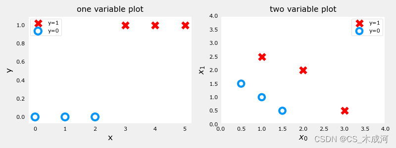
由上图可以看到，在单变量图中，positive显示为红色，y=1；negative显示为蓝色，y=0。在线性回归中，y的值不局限于两个值，可以是任意值。在多变量图中，同样地，positive显示为红色，negative显示为蓝色。在具有多个变量的线性回归的情况下，y不会被限制为两个值，类似的图将是三维的。

2. 线性回归方法

这里，我们使用前面介绍的线性回归模型根据肿瘤大小预测肿瘤是良性还是恶性。

w_in = np.zeros((1))
b_in = 0
plt.close('all') 
addpt = plt_one_addpt_onclick( x_train,y_train, w_in, b_in, logistic=False)

在这里插入图片描述
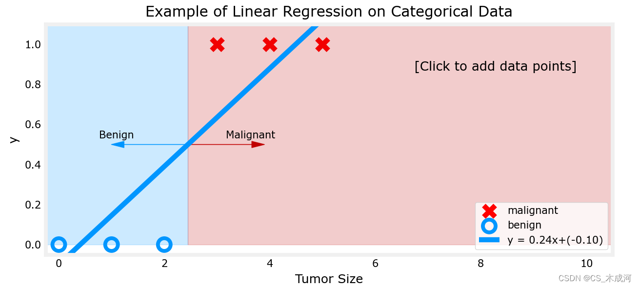
其中，阈值为0.5

现在，在大肿瘤大小范围（接近10）的最右侧添加更多的“恶性”数据点，并重新运行线性回归。
在这里插入图片描述
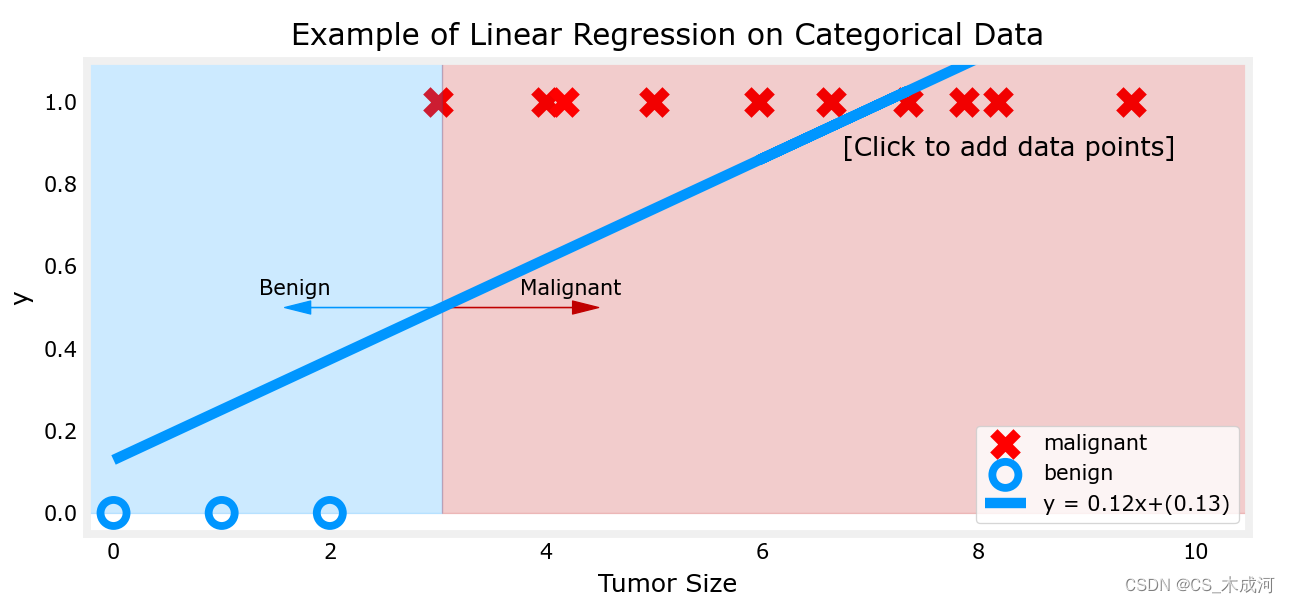
该模型预测了更大的肿瘤，但x=3的数据点被错误地预测了。

上面的例子表明，线性模型不足以对分类数据进行建模。

3. 逻辑函数（sigmod）

sigmod函数公式表示为：
$\frac{1}{1+e^{-z}} \tag{1}$
其中， $z$ 是sigmod函数的输入，一个线性回归模型的输出。在单变量线性回归中，它是标量；在多变量线性回归中，它可能是包含 $m$ 个值的向量。

sigmoid函数的实现如下：

def sigmoid(z):"""Compute the sigmoid of zArgs:z (ndarray): A scalar, numpy array of any size.Returns:g (ndarray): sigmoid(z), with the same shape as z"""g = 1/(1+np.exp(-z))return g

对于输入变量 $z$ ，输出结果为：

# Generate an array of evenly spaced values between -10 and 10
z_tmp = np.arange(-10,11)# Use the function implemented above to get the sigmoid values
y = sigmoid(z_tmp)# Code for pretty printing the two arrays next to each other
np.set_printoptions(precision=3) 
print("Input (z), Output (sigmoid(z))")
print(np.c_[z_tmp, y])

在这里插入图片描述
左边是输入z，右边是输出sigmod(z).输入值的范围从-10到10，输出值的范围从0到1.

对结果进行可视化：

# Plot z vs sigmoid(z)
fig,ax = plt.subplots(1,1,figsize=(5,3))
ax.plot(z_tmp, y, c="b")ax.set_title("Sigmoid function")
ax.set_ylabel('sigmoid(z)')
ax.set_xlabel('z')
draw_vthresh(ax,0)

在这里插入图片描述
从图中可以看出，sigmod函数在z取小负数时趋近于0，在z取大正数时趋近于1.

4.逻辑回归

逻辑回归模型将sigmod函数应用到线性回归模型中，如下所示：
$f_{\mathbf{w},b}(\mathbf{x}^{(i)}) = g(\mathbf{w} \cdot \mathbf{x}^{(i)} + b ) \tag{2}$
其中，
$\frac{1}{1+e^{-z}}\tag{3}$

将逻辑回归应用到肿瘤分类的例子中。

首先，加载样例和初始化参数。

x_train = np.array([0., 1, 2, 3, 4, 5])
y_train = np.array([0,  0, 0, 1, 1, 1])w_in = np.zeros((1))
b_in = 0

plt.close('all') 
addpt = plt_one_addpt_onclick( x_train,y_train, w_in, b_in, logistic=True)

在这里插入图片描述
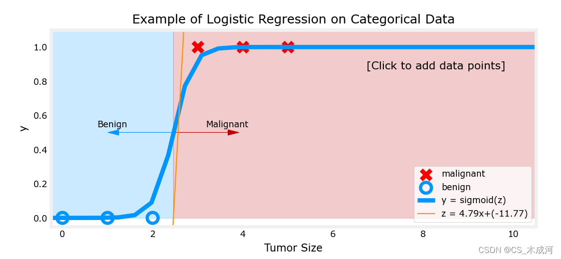
其中，橘黄色线是 $z$ 或者 $\mathbf{w} \cdot \mathbf{x}^{(i)} + b$ ，阈值为0.5

现在，在大肿瘤大小范围（接近10）中添加更多的数据点，并重新运行。
在这里插入图片描述
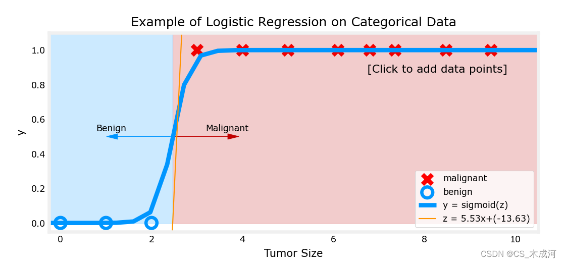
与线性回归模型不同，该模型继续做出正确的预测。

5. 决策边界

5.1 数据集

X = np.array([[0.5, 1.5], [1,1], [1.5, 0.5], [3, 0.5], [2, 2], [1, 2.5]])
y = np.array([0, 0, 0, 1, 1, 1]).reshape(-1,1)

5.2 数据绘图

fig,ax = plt.subplots(1,1,figsize=(4,4))
plot_data(X, y, ax)ax.axis([0, 4, 0, 3.5])
ax.set_ylabel('$x_1$')
ax.set_xlabel('$x_0$')
plt.show()

在这里插入图片描述

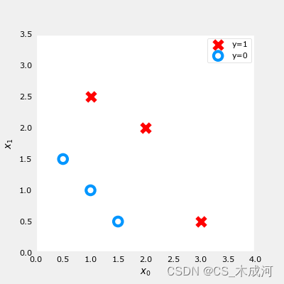
我们要根据数据集训练一个逻辑回归模型，其公式为： $f(x) = g(w_0x_0+w_1x_1 + b)$ ，其中 $\frac{1}{1+e^{-z}}$ , 训练好模型得到参数 $b = -3, w_0 = 1, w_1 = 1$ . 即 $f(x) = g(x_0+x_1-3)$ 。下面通过绘制决策边界来了解这个经过训练的模型在预测什么。

5.3 逻辑回归与决策边界的刷新

逻辑回归模型表示为：
$f_{\mathbf{w},b}(\mathbf{x}^{(i)}) = g(\mathbf{w} \cdot \mathbf{x}^{(i)} + b) \tag{1}$

其中， $g (z)$ 是 sigmoid 函数，它可以将所有值映射到0到1之间:
$\frac{1}{1+e^{-z}}\tag{2}$
$\mathbf{w} \cdot \mathbf{x}$ 是向量点积运算:
$\mathbf{w} \cdot \mathbf{x} = w_0 x_0 + w_1 x_1$

我们把模型的输出( $f_{\mathbf{w},b}(x)$ ) 解释为给定 $x$ 并由 $w$ 和 $b$ 参数化的 $y = 1$ 的概率.
这样, 为了从逻辑回归模型中获得最终预测 ( $y = 0$ or $y = 1$ ) ，使用以下启发式：
if $f_{\mathbf{w},b}(x) >= 0.5$ , predict $y = 1$
if $f_{\mathbf{w},b}(x) < 0.5$ , predict $y = 0$
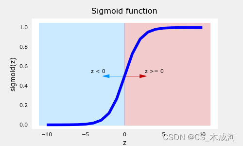
绘制sigmoid 函数来看看哪里 $g (z) >= 0.5$

# Plot sigmoid(z) over a range of values from -10 to 10
z = np.arange(-10,11)fig,ax = plt.subplots(1,1,figsize=(5,3))
# Plot z vs sigmoid(z)
ax.plot(z, sigmoid(z), c="b")ax.set_title("Sigmoid function")
ax.set_ylabel('sigmoid(z)')
ax.set_xlabel('z')
draw_vthresh(ax,0)

在这里插入图片描述

如图所示，当 $z >= 0$ 时, $g (z) >= 0.5$
对于逻辑回归模型, $\mathbf{w} \cdot \mathbf{x} + b$ . 因此,

if $\mathbf{w} \cdot \mathbf{x} + b >= 0$ , 模型预测 $y = 1$

if $\mathbf{w} \cdot \mathbf{x} + b < 0$ , 模型预测 $y = 0$

5.4 绘制决策边界

现在，我们回到例子中理解逻辑回归模型是如何预测的.

我们的逻辑回归模型为：
$f(x) = g(-3 + x_0+x_1)$
从上面所讲，可以知道 if $3 + x_0+x_1 >= 0$ ，模型预测 $y = 1$

通过绘图来可视化。从绘制 $3+x_0+x_1=0$ 开始，这相当于 $x_1=3-x_0$ 。

# Choose values between 0 and 6
x0 = np.arange(0,6)x1 = 3 - x0
fig,ax = plt.subplots(1,1,figsize=(5,4))
# Plot the decision boundary
ax.plot(x0,x1, c="b")
ax.axis([0, 4, 0, 3.5])# Fill the region below the line
ax.fill_between(x0,x1, alpha=0.2)# Plot the original data
plot_data(X,y,ax)
ax.set_ylabel(r'$x_1$')
ax.set_xlabel(r'$x_0$')
plt.show()

在这里插入图片描述

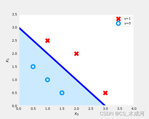
在上图中，蓝线表示 $x_0+x_1-3=0$ ，它应该在3处与 $x_1$ 轴相交（如果我们设置 $x_1$ =3， $x_0$ =0），并且在3处相交 $x_0$ 轴（如果我们将 $x_1$ 设置为0， $x_0$ =3）。
阴影区域表示 $3+x_0+x_1<0$ 。该线上方的区域为 $3+x_0+x_1>0$ 。
阴影区域（线下）中的任何点都被分类为 $y = 0$ 。该线上或上方的任何点都被分类为 $y = 1$ 。这条线被称为“决策边界”。

通过使用高阶多项式项（例如： $f(x) = g( x_0^2 + x_1 -1)$ ），我们可以得出更复杂的非线性边界。

附录

lab_utils_common.py 源码：

"""
lab_utils_commoncontains common routines and variable definitionsused by all the labs in this week.by contrast, specific, large plotting routines will be in separate filesand are generally imported into the week where they are used.those files will import this file
"""
import copy
import math
import numpy as np
import matplotlib.pyplot as plt
from matplotlib.patches import FancyArrowPatch
from ipywidgets import Outputnp.set_printoptions(precision=2)dlc = dict(dlblue = '#0096ff', dlorange = '#FF9300', dldarkred='#C00000', dlmagenta='#FF40FF', dlpurple='#7030A0')
dlblue = '#0096ff'; dlorange = '#FF9300'; dldarkred='#C00000'; dlmagenta='#FF40FF'; dlpurple='#7030A0'
dlcolors = [dlblue, dlorange, dldarkred, dlmagenta, dlpurple]
plt.style.use('./deeplearning.mplstyle')def sigmoid(z):"""Compute the sigmoid of zParameters----------z : array_likeA scalar or numpy array of any size.Returns-------g : array_likesigmoid(z)"""z = np.clip( z, -500, 500 )           # protect against overflowg = 1.0/(1.0+np.exp(-z))return g##########################################################
# Regression Routines
##########################################################def predict_logistic(X, w, b):""" performs prediction """return sigmoid(X @ w + b)def predict_linear(X, w, b):""" performs prediction """return X @ w + bdef compute_cost_logistic(X, y, w, b, lambda_=0, safe=False):"""Computes cost using logistic loss, non-matrix versionArgs:X (ndarray): Shape (m,n)  matrix of examples with n featuresy (ndarray): Shape (m,)   target valuesw (ndarray): Shape (n,)   parameters for predictionb (scalar):               parameter  for predictionlambda_ : (scalar, float) Controls amount of regularization, 0 = no regularizationsafe : (boolean)          True-selects under/overflow safe algorithmReturns:cost (scalar): cost"""m,n = X.shapecost = 0.0for i in range(m):z_i    = np.dot(X[i],w) + b                                             #(n,)(n,) or (n,) ()if safe:  #avoids overflowscost += -(y[i] * z_i ) + log_1pexp(z_i)else:f_wb_i = sigmoid(z_i)                                                   #(n,)cost  += -y[i] * np.log(f_wb_i) - (1 - y[i]) * np.log(1 - f_wb_i)       # scalarcost = cost/mreg_cost = 0if lambda_ != 0:for j in range(n):reg_cost += (w[j]**2)                                               # scalarreg_cost = (lambda_/(2*m))*reg_costreturn cost + reg_costdef log_1pexp(x, maximum=20):''' approximate log(1+exp^x)https://stats.stackexchange.com/questions/475589/numerical-computation-of-cross-entropy-in-practiceArgs:x   : (ndarray Shape (n,1) or (n,)  inputout : (ndarray Shape matches x      output ~= np.log(1+exp(x))'''out  = np.zeros_like(x,dtype=float)i    = x <= maximumni   = np.logical_not(i)out[i]  = np.log(1 + np.exp(x[i]))out[ni] = x[ni]return outdef compute_cost_matrix(X, y, w, b, logistic=False, lambda_=0, safe=True):"""Computes the cost using  using matricesArgs:X : (ndarray, Shape (m,n))          matrix of examplesy : (ndarray  Shape (m,) or (m,1))  target value of each examplew : (ndarray  Shape (n,) or (n,1))  Values of parameter(s) of the modelb : (scalar )                       Values of parameter of the modelverbose : (Boolean) If true, print out intermediate value f_wbReturns:total_cost: (scalar)                cost"""m = X.shape[0]y = y.reshape(-1,1)             # ensure 2Dw = w.reshape(-1,1)             # ensure 2Dif logistic:if safe:  #safe from overflowz = X @ w + b                                                           #(m,n)(n,1)=(m,1)cost = -(y * z) + log_1pexp(z)cost = np.sum(cost)/m                                                   # (scalar)else:f    = sigmoid(X @ w + b)                                               # (m,n)(n,1) = (m,1)cost = (1/m)*(np.dot(-y.T, np.log(f)) - np.dot((1-y).T, np.log(1-f)))   # (1,m)(m,1) = (1,1)cost = cost[0,0]                                                        # scalarelse:f    = X @ w + b                                                        # (m,n)(n,1) = (m,1)cost = (1/(2*m)) * np.sum((f - y)**2)                                   # scalarreg_cost = (lambda_/(2*m)) * np.sum(w**2)                                   # scalartotal_cost = cost + reg_cost                                                # scalarreturn total_cost                                                           # scalardef compute_gradient_matrix(X, y, w, b, logistic=False, lambda_=0):"""Computes the gradient using matricesArgs:X : (ndarray, Shape (m,n))          matrix of examplesy : (ndarray  Shape (m,) or (m,1))  target value of each examplew : (ndarray  Shape (n,) or (n,1))  Values of parameters of the modelb : (scalar )                       Values of parameter of the modellogistic: (boolean)                 linear if false, logistic if truelambda_:  (float)                   applies regularization if non-zeroReturnsdj_dw: (array_like Shape (n,1))     The gradient of the cost w.r.t. the parameters wdj_db: (scalar)                     The gradient of the cost w.r.t. the parameter b"""m = X.shape[0]y = y.reshape(-1,1)             # ensure 2Dw = w.reshape(-1,1)             # ensure 2Df_wb  = sigmoid( X @ w + b ) if logistic else  X @ w + b      # (m,n)(n,1) = (m,1)err   = f_wb - y                                              # (m,1)dj_dw = (1/m) * (X.T @ err)                                   # (n,m)(m,1) = (n,1)dj_db = (1/m) * np.sum(err)                                   # scalardj_dw += (lambda_/m) * w        # regularize                  # (n,1)return dj_db, dj_dw                                           # scalar, (n,1)def gradient_descent(X, y, w_in, b_in, alpha, num_iters, logistic=False, lambda_=0, verbose=True):"""Performs batch gradient descent to learn theta. Updates theta by takingnum_iters gradient steps with learning rate alphaArgs:X (ndarray):    Shape (m,n)         matrix of examplesy (ndarray):    Shape (m,) or (m,1) target value of each examplew_in (ndarray): Shape (n,) or (n,1) Initial values of parameters of the modelb_in (scalar):                      Initial value of parameter of the modellogistic: (boolean)                 linear if false, logistic if truelambda_:  (float)                   applies regularization if non-zeroalpha (float):                      Learning ratenum_iters (int):                    number of iterations to run gradient descentReturns:w (ndarray): Shape (n,) or (n,1)    Updated values of parameters; matches incoming shapeb (scalar):                         Updated value of parameter"""# An array to store cost J and w's at each iteration primarily for graphing laterJ_history = []w = copy.deepcopy(w_in)  #avoid modifying global w within functionb = b_inw = w.reshape(-1,1)      #prep for matrix operationsy = y.reshape(-1,1)for i in range(num_iters):# Calculate the gradient and update the parametersdj_db,dj_dw = compute_gradient_matrix(X, y, w, b, logistic, lambda_)# Update Parameters using w, b, alpha and gradientw = w - alpha * dj_dwb = b - alpha * dj_db# Save cost J at each iterationif i<100000:      # prevent resource exhaustionJ_history.append( compute_cost_matrix(X, y, w, b, logistic, lambda_) )# Print cost every at intervals 10 times or as many iterations if < 10if i% math.ceil(num_iters / 10) == 0:if verbose: print(f"Iteration {i:4d}: Cost {J_history[-1]}   ")return w.reshape(w_in.shape), b, J_history  #return final w,b and J history for graphingdef zscore_normalize_features(X):"""computes  X, zcore normalized by columnArgs:X (ndarray): Shape (m,n) input data, m examples, n featuresReturns:X_norm (ndarray): Shape (m,n)  input normalized by columnmu (ndarray):     Shape (n,)   mean of each featuresigma (ndarray):  Shape (n,)   standard deviation of each feature"""# find the mean of each column/featuremu     = np.mean(X, axis=0)                 # mu will have shape (n,)# find the standard deviation of each column/featuresigma  = np.std(X, axis=0)                  # sigma will have shape (n,)# element-wise, subtract mu for that column from each example, divide by std for that columnX_norm = (X - mu) / sigmareturn X_norm, mu, sigma#check our work
#from sklearn.preprocessing import scale
#scale(X_orig, axis=0, with_mean=True, with_std=True, copy=True)######################################################
# Common Plotting Routines
######################################################def plot_data(X, y, ax, pos_label="y=1", neg_label="y=0", s=80, loc='best' ):""" plots logistic data with two axis """# Find Indices of Positive and Negative Examplespos = y == 1neg = y == 0pos = pos.reshape(-1,)  #work with 1D or 1D y vectorsneg = neg.reshape(-1,)# Plot examplesax.scatter(X[pos, 0], X[pos, 1], marker='x', s=s, c = 'red', label=pos_label)ax.scatter(X[neg, 0], X[neg, 1], marker='o', s=s, label=neg_label, facecolors='none', edgecolors=dlblue, lw=3)ax.legend(loc=loc)ax.figure.canvas.toolbar_visible = Falseax.figure.canvas.header_visible = Falseax.figure.canvas.footer_visible = Falsedef plt_tumor_data(x, y, ax):""" plots tumor data on one axis """pos = y == 1neg = y == 0ax.scatter(x[pos], y[pos], marker='x', s=80, c = 'red', label="malignant")ax.scatter(x[neg], y[neg], marker='o', s=100, label="benign", facecolors='none', edgecolors=dlblue,lw=3)ax.set_ylim(-0.175,1.1)ax.set_ylabel('y')ax.set_xlabel('Tumor Size')ax.set_title("Logistic Regression on Categorical Data")ax.figure.canvas.toolbar_visible = Falseax.figure.canvas.header_visible = Falseax.figure.canvas.footer_visible = False# Draws a threshold at 0.5
def draw_vthresh(ax,x):""" draws a threshold """ylim = ax.get_ylim()xlim = ax.get_xlim()ax.fill_between([xlim[0], x], [ylim[1], ylim[1]], alpha=0.2, color=dlblue)ax.fill_between([x, xlim[1]], [ylim[1], ylim[1]], alpha=0.2, color=dldarkred)ax.annotate("z >= 0", xy= [x,0.5], xycoords='data',xytext=[30,5],textcoords='offset points')d = FancyArrowPatch(posA=(x, 0.5), posB=(x+3, 0.5), color=dldarkred,arrowstyle='simple, head_width=5, head_length=10, tail_width=0.0',)ax.add_artist(d)ax.annotate("z < 0", xy= [x,0.5], xycoords='data',xytext=[-50,5],textcoords='offset points', ha='left')f = FancyArrowPatch(posA=(x, 0.5), posB=(x-3, 0.5), color=dlblue,arrowstyle='simple, head_width=5, head_length=10, tail_width=0.0',)ax.add_artist(f)

plt_one_addpt_onclick.py 源码：

import time
import copy
from ipywidgets import Output
from matplotlib.widgets import Button, CheckButtons
from matplotlib.patches import FancyArrowPatch
from lab_utils_common import np, plt, dlblue, dlorange, sigmoid, dldarkred, gradient_descent# for debug
#output = Output() # sends hidden error messages to display when using widgets
#display(output)class plt_one_addpt_onclick:""" class to run one interactive plot """def __init__(self, x, y, w, b, logistic=True):self.logistic=logisticpos = y == 1neg = y == 0fig,ax = plt.subplots(1,1,figsize=(8,4))fig.canvas.toolbar_visible = Falsefig.canvas.header_visible = Falsefig.canvas.footer_visible = Falseplt.subplots_adjust(bottom=0.25)ax.scatter(x[pos], y[pos], marker='x', s=80, c = 'red', label="malignant")ax.scatter(x[neg], y[neg], marker='o', s=100, label="benign", facecolors='none', edgecolors=dlblue,lw=3)ax.set_ylim(-0.05,1.1)xlim = ax.get_xlim()ax.set_xlim(xlim[0],xlim[1]*2)ax.set_ylabel('y')ax.set_xlabel('Tumor Size')self.alegend = ax.legend(loc='lower right')if self.logistic:ax.set_title("Example of Logistic Regression on Categorical Data")else:ax.set_title("Example of Linear Regression on Categorical Data")ax.text(0.65,0.8,"[Click to add data points]", size=10, transform=ax.transAxes)axcalc   = plt.axes([0.1, 0.05, 0.38, 0.075])  #l,b,w,haxthresh = plt.axes([0.5, 0.05, 0.38, 0.075])  #l,b,w,hself.tlist = []self.fig = figself.ax = [ax,axcalc,axthresh]self.x = xself.y = yself.w = copy.deepcopy(w)self.b = bf_wb = np.matmul(self.x.reshape(-1,1), self.w) + self.bif self.logistic:self.aline = self.ax[0].plot(self.x, sigmoid(f_wb), color=dlblue)self.bline = self.ax[0].plot(self.x, f_wb, color=dlorange,lw=1)else:self.aline = self.ax[0].plot(self.x, sigmoid(f_wb), color=dlblue)self.cid = fig.canvas.mpl_connect('button_press_event', self.add_data)if self.logistic:self.bcalc = Button(axcalc, 'Run Logistic Regression (click)', color=dlblue)self.bcalc.on_clicked(self.calc_logistic)else:self.bcalc = Button(axcalc, 'Run Linear Regression (click)', color=dlblue)self.bcalc.on_clicked(self.calc_linear)self.bthresh = CheckButtons(axthresh, ('Toggle 0.5 threshold (after regression)',))self.bthresh.on_clicked(self.thresh)self.resize_sq(self.bthresh)#   @output.capture()  # debugdef add_data(self, event):#self.ax[0].text(0.1,0.1, f"in onclick")if event.inaxes == self.ax[0]:x_coord = event.xdatay_coord = event.ydataif y_coord > 0.5:self.ax[0].scatter(x_coord, 1, marker='x', s=80, c = 'red' )self.y = np.append(self.y,1)else:self.ax[0].scatter(x_coord, 0, marker='o', s=100, facecolors='none', edgecolors=dlblue,lw=3)self.y = np.append(self.y,0)self.x = np.append(self.x,x_coord)self.fig.canvas.draw()#   @output.capture()  # debugdef calc_linear(self, event):if self.bthresh.get_status()[0]:self.remove_thresh()for it in [1,1,1,1,1,2,4,8,16,32,64,128,256]:self.w, self.b, _ = gradient_descent(self.x.reshape(-1,1), self.y.reshape(-1,1),self.w.reshape(-1,1), self.b, 0.01, it,logistic=False, lambda_=0, verbose=False)self.aline[0].remove()self.alegend.remove()y_hat = np.matmul(self.x.reshape(-1,1), self.w) + self.bself.aline = self.ax[0].plot(self.x, y_hat, color=dlblue,label=f"y = {np.squeeze(self.w):0.2f}x+({self.b:0.2f})")self.alegend = self.ax[0].legend(loc='lower right')time.sleep(0.3)self.fig.canvas.draw()if self.bthresh.get_status()[0]:self.draw_thresh()self.fig.canvas.draw()def calc_logistic(self, event):if self.bthresh.get_status()[0]:self.remove_thresh()for it in [1, 8,16,32,64,128,256,512,1024,2048,4096]:self.w, self.b, _ = gradient_descent(self.x.reshape(-1,1), self.y.reshape(-1,1),self.w.reshape(-1,1), self.b, 0.1, it,logistic=True, lambda_=0, verbose=False)self.aline[0].remove()self.bline[0].remove()self.alegend.remove()xlim  = self.ax[0].get_xlim()x_hat = np.linspace(*xlim, 30)y_hat = sigmoid(np.matmul(x_hat.reshape(-1,1), self.w) + self.b)self.aline = self.ax[0].plot(x_hat, y_hat, color=dlblue,label="y = sigmoid(z)")f_wb = np.matmul(x_hat.reshape(-1,1), self.w) + self.bself.bline = self.ax[0].plot(x_hat, f_wb, color=dlorange, lw=1,label=f"z = {np.squeeze(self.w):0.2f}x+({self.b:0.2f})")self.alegend = self.ax[0].legend(loc='lower right')time.sleep(0.3)self.fig.canvas.draw()if self.bthresh.get_status()[0]:self.draw_thresh()self.fig.canvas.draw()def thresh(self, event):if self.bthresh.get_status()[0]:#plt.figtext(0,0, f"in thresh {self.bthresh.get_status()}")self.draw_thresh()else:#plt.figtext(0,0.3, f"in thresh {self.bthresh.get_status()}")self.remove_thresh()def draw_thresh(self):ws = np.squeeze(self.w)xp5 = -self.b/ws if self.logistic else (0.5 - self.b) / wsylim = self.ax[0].get_ylim()xlim = self.ax[0].get_xlim()a = self.ax[0].fill_between([xlim[0], xp5], [ylim[1], ylim[1]], alpha=0.2, color=dlblue)b = self.ax[0].fill_between([xp5, xlim[1]], [ylim[1], ylim[1]], alpha=0.2, color=dldarkred)c = self.ax[0].annotate("Malignant", xy= [xp5,0.5], xycoords='data',xytext=[30,5],textcoords='offset points')d = FancyArrowPatch(posA=(xp5, 0.5), posB=(xp5+1.5, 0.5), color=dldarkred,arrowstyle='simple, head_width=5, head_length=10, tail_width=0.0',)self.ax[0].add_artist(d)e = self.ax[0].annotate("Benign", xy= [xp5,0.5], xycoords='data',xytext=[-70,5],textcoords='offset points', ha='left')f = FancyArrowPatch(posA=(xp5, 0.5), posB=(xp5-1.5, 0.5), color=dlblue,arrowstyle='simple, head_width=5, head_length=10, tail_width=0.0',)self.ax[0].add_artist(f)self.tlist = [a,b,c,d,e,f]self.fig.canvas.draw()def remove_thresh(self):#plt.figtext(0.5,0.0, f"rem thresh {self.bthresh.get_status()}")for artist in self.tlist:artist.remove()self.fig.canvas.draw()def resize_sq(self, bcid):""" resizes the check box """#future reference#print(f"width  : {bcid.rectangles[0].get_width()}")#print(f"height : {bcid.rectangles[0].get_height()}")#print(f"xy     : {bcid.rectangles[0].get_xy()}")#print(f"bb     : {bcid.rectangles[0].get_bbox()}")#print(f"points : {bcid.rectangles[0].get_bbox().get_points()}")  #[[xmin,ymin],[xmax,ymax]]h = bcid.rectangles[0].get_height()bcid.rectangles[0].set_height(3*h)ymax = bcid.rectangles[0].get_bbox().y1ymin = bcid.rectangles[0].get_bbox().y0bcid.lines[0][0].set_ydata([ymax,ymin])bcid.lines[0][1].set_ydata([ymin,ymax])